$$ % ASYMPTOTIC NOTATIONS \newcommand{\BigO}{\mathcal{O}} % NUMBER SYSTEMS \newcommand{\A}{\mathbb{A}} \newcommand{\B}{\mathbb{B}} \newcommand{\C}{\mathbb{C}} \newcommand{\D}{\mathbb{D}} \newcommand{\E}{\mathbb{E}} \newcommand{\F}{\mathbb{F}} \newcommand{\G}{\mathbb{G}} %\newcommand{\bbH}{\mathbb{H}} \newcommand{\I}{\mathbb{I}} \newcommand{\J}{\mathbb{J}} \newcommand{\K}{\mathbb{K}} %\newcommand{\bbL}{\mathbb{L}} \newcommand{\M}{\mathbb{M}} \newcommand{\N}{\mathbb{N}} %\newcommand{\bbO}{\mathbb{O}} %\newcommand{\bbP}{\mathbb{P}} \newcommand{\Q}{\mathbb{Q}} \newcommand{\R}{\mathbb{R}} %\newcommand{\bbS}{\mathbb{S}} %\newcommand{\bbT}{\mathbb{T}} \newcommand{\U}{\mathbb{U}} \newcommand{\V}{\mathbb{V}} \newcommand{\W}{\mathbb{W}} \newcommand{\X}{\mathbb{X}} \newcommand{\Y}{\mathbb{Y}} \newcommand{\Z}{\mathbb{Z}} \newcommand{\bbA}{\mathbb{A}} \newcommand{\bbB}{\mathbb{B}} \newcommand{\bbC}{\mathbb{C}} \newcommand{\bbD}{\mathbb{D}} \newcommand{\bbE}{\mathbb{E}} \newcommand{\bbF}{\mathbb{F}} \newcommand{\bbG}{\mathbb{G}} \newcommand{\bbH}{\mathbb{H}} \newcommand{\bbI}{\mathbb{I}} \newcommand{\bbJ}{\mathbb{J}} \newcommand{\bbK}{\mathbb{K}} \newcommand{\bbL}{\mathbb{L}} \newcommand{\bbM}{\mathbb{M}} \newcommand{\bbN}{\mathbb{N}} \newcommand{\bbO}{\mathbb{O}} \newcommand{\bbP}{\mathbb{P}} \newcommand{\bbQ}{\mathbb{Q}} \newcommand{\bbR}{\mathbb{R}} \newcommand{\bbS}{\mathbb{S}} \newcommand{\bbT}{\mathbb{T}} \newcommand{\bbU}{\mathbb{U}} \newcommand{\bbV}{\mathbb{V}} \newcommand{\bbW}{\mathbb{W}} \newcommand{\bbX}{\mathbb{X}} \newcommand{\bbY}{\mathbb{Y}} \newcommand{\bbZ}{\mathbb{Z}} % CALLICGRAPHIC SHORTCUTS \newcommand{\cA}{\mathcal{A}} \newcommand{\cB}{\mathcal{B}} \newcommand{\cC}{\mathcal{C}} \newcommand{\cD}{\mathcal{D}} \newcommand{\cE}{\mathcal{E}} \newcommand{\cF}{\mathcal{F}} \newcommand{\cG}{\mathcal{G}} \newcommand{\cH}{\mathcal{H}} \newcommand{\cI}{\mathcal{I}} \newcommand{\cJ}{\mathcal{J}} \newcommand{\cK}{\mathcal{K}} \newcommand{\cL}{\mathcal{L}} \newcommand{\cM}{\mathcal{M}} \newcommand{\cN}{\mathcal{N}} \newcommand{\cO}{\mathcal{O}} \newcommand{\cP}{\mathcal{P}} \newcommand{\cQ}{\mathcal{Q}} \newcommand{\cR}{\mathcal{R}} \newcommand{\cS}{\mathcal{S}} \newcommand{\cT}{\mathcal{T}} \newcommand{\cU}{\mathcal{U}} \newcommand{\cV}{\mathcal{V}} \newcommand{\cW}{\mathcal{W}} \newcommand{\cX}{\mathcal{X}} \newcommand{\cY}{\mathcal{Y}} \newcommand{\cZ}{\mathcal{Z}} % BRACES \newcommand{\set}[1]{\left\{ #1 \right\}} \newcommand{\dset}[2]{\left\{ #1 \ \middle| \ #2 \right\}} \newcommand{\alg}[1]{\left\langle #1 \right\rangle} \newcommand{\card}[1]{\left\lvert #1 \right\rvert} \newcommand{\length}[1]{\left\lvert #1 \right\rvert} \newcommand{\abs}[1]{\left\lvert #1 \right\rvert} \renewcommand{\mag}[1]{\left\lvert #1 \right\rvert} \newcommand{\norm}[1]{\left\lVert #1 \right\rVert} \newcommand{\scprod}[1]{\left\langle #1 \right\rangle} \newcommand{\ceil}[1]{\left\lceil #1 \right\rceil} \newcommand{\floor}[1]{\left\lfloor #1 \right\rfloor} \newcommand{\linsys}[2]{\left[\ #1 \ \middle| \ #2 \ \right]} \newcommand{\Sim}[1]{\text{Sim}\left( #1 \right)} \newcommand{\Tr}[1]{\mathsf{Tr}\left( #1 \right)} \newcommand{\bra}[1]{\left\langle #1 \right\rvert} \newcommand{\ket}[1]{\left\lvert #1 \right\rangle} \newcommand{\bracket}[2]{\left\langle #1 \ \middle| \ #2 \right\rangle} % BRACES SMALL (no adjusting) \newcommand{\sset}[1]{\{ #1 \}} \newcommand{\sdset}[2]{\{ #1 \ | \ #2 \}} \newcommand{\salg}[1]{\langle #1 \rangle} \newcommand{\scard}[1]{\lvert #1 \rvert} \newcommand{\slength}[1]{\lvert #1 \rvert} \newcommand{\sabs}[1]{\lvert #1 \rvert} \newcommand{\smag}[1]{\lvert #1 \rvert} \newcommand{\snorm}[1]{\lVert #1 \rVert} \newcommand{\sscprod}[1]{\langle #1 \rangle} \newcommand{\sceil}[1]{\lceil #1 \rceil} \newcommand{\sfloor}[1]{\lfloor #1 \rfloor} \newcommand{\slinsys}[2]{[\ #1 \ | \ #2 \ ]} \newcommand{\sSim}[1]{\text{Sim}( #1 )} \newcommand{\sTr}[1]{\mathsf{Tr}( #1 )} \newcommand{\sbra}[1]{\langle #1 \rvert} \newcommand{\sket}[1]{\lvert #1 \rangle} \newcommand{\sbracket}[2]{\langle #1 \ | \ #2 \rangle} % OPERATORS \newcommand{\conv}{*} \newcommand{\proj}{\text{proj}} % EMPTY SET \let\oldemptyset\emptyset \let\emptyset\varnothing % NOT IN SHORTCUT \newcommand{\nin}{\not\in} % CUSTOM STATISTICS AND PROBABILITY \newcommand{\Prob}[2][]{P_{#1}\left( #2 \right)} \newcommand{\cProb}[3][]{P_{#1}\left( #2 \,\middle|\, #3 \right)} \newcommand{\Dist}[2]{#1\left( #2 \right)} \newcommand{\cDist}[3]{#1\left( #2 \,\middle|\, #3 \right)} \newcommand{\hProb}[2][]{\hat{P}_{#1}\left( #2 \right)} \newcommand{\chProb}[2]{\hat{P}\left( #1 \,\middle|\, #2 \right)} \newcommand{\Var}[2][]{\operatorname{Var}_{#1}\left[ #2 \right]} \newcommand{\sd}[1]{\operatorname{sd}\left( #1 \right)} \newcommand{\Exp}[2][]{\mathbb{E}_{#1}\left[ #2 \right]} \newcommand{\cExp}[3][]{\mathbb{E}_{#1}\left[ #2 \,\middle|\, #3 \right]} \newcommand{\hExp}[2][]{\mathbb{\hat{E}_{#1}}\left[ #2 \right]} \newcommand{\chExp}[3][]{\mathbb{\hat{E}}_{#1}\left[ #2 \,\middle|\, #3 \right]} \newcommand{\Corr}[1]{\operatorname{Corr}\left[ #1 \right]} \newcommand{\Cov}[1]{\operatorname{Cov}\left(#1 \right)} \newcommand{\MSE}[2][]{\operatorname{MSE}_{#1}\left[ #2 \right]} \newcommand{\riid}{\stackrel{\text{i.i.d.}}{\sim}} \newcommand{\approxsim}{\stackrel{\text{approx.}}{\sim}} \newcommand{\ind}[1]{\mathbb{1}_{\set{#1}}} \newcommand{\eqiid}{\stackrel{\text{\tiny i.i.d.}}{=}} \newcommand{\eqind}{\stackrel{\text{\tiny ind.}}{=}} % BAYESIAN NETWORKS \newcommand{\indep}{\perp} \newcommand{\given}{\,\,|\,\,} \newcommand{\Pa}{\mathbf{Pa}} \newcommand{\dsep}[2]{\operatorname{d-sep}\left( #1 \,\middle|\, #2 \right)} % RANDOM VARIABLES \newcommand{\rA}{A} \newcommand{\rB}{B} \newcommand{\rC}{C} \newcommand{\rD}{D} \newcommand{\rE}{E} \newcommand{\rF}{F} \newcommand{\rG}{G} \newcommand{\rH}{H} \newcommand{\rI}{I} \newcommand{\rJ}{J} \newcommand{\rK}{K} \newcommand{\rL}{L} \newcommand{\rM}{M} \newcommand{\rN}{N} \newcommand{\rO}{O} \newcommand{\rP}{P} \newcommand{\rQ}{Q} \newcommand{\rR}{R} \newcommand{\rS}{S} \newcommand{\rT}{T} \newcommand{\rU}{U} \newcommand{\rV}{V} \newcommand{\rW}{W} \newcommand{\rX}{X} \newcommand{\rY}{Y} \newcommand{\rZ}{Z} % RANDOM VECTORS % declares a custom italic bold alphabet for random vectors \DeclareMathAlphabet{\mathbfit}{OML}{cmm}{b}{it} \newcommand{\rvA}{\mathbfit{A}} \newcommand{\rvB}{\mathbfit{B}} \newcommand{\rvC}{\mathbfit{C}} \newcommand{\rvD}{\mathbfit{D}} \newcommand{\rvE}{\mathbfit{E}} \newcommand{\rvF}{\mathbfit{F}} \newcommand{\rvG}{\mathbfit{G}} \newcommand{\rvH}{\mathbfit{H}} \newcommand{\rvI}{\mathbfit{I}} \newcommand{\rvJ}{\mathbfit{J}} \newcommand{\rvK}{\mathbfit{K}} \newcommand{\rvL}{\mathbfit{L}} \newcommand{\rvM}{\mathbfit{M}} \newcommand{\rvN}{\mathbfit{N}} \newcommand{\rvO}{\mathbfit{O}} \newcommand{\rvP}{\mathbfit{P}} \newcommand{\rvQ}{\mathbfit{Q}} \newcommand{\rvR}{\mathbfit{R}} \newcommand{\rvS}{\mathbfit{S}} \newcommand{\rvT}{\mathbfit{T}} \newcommand{\rvU}{\mathbfit{U}} \newcommand{\rvV}{\mathbfit{V}} \newcommand{\rvW}{\mathbfit{W}} \newcommand{\rvX}{\mathbfit{X}} \newcommand{\rvY}{\mathbfit{Y}} \newcommand{\rvZ}{\mathbfit{Z}} % MACHINE LEARNING \newcommand{\Risk}[1]{R\left(#1\right)} \newcommand{\empRisk}[1]{\widehat{R}\left(#1\right)} % RECOMMENDER SYSTEMS \newcommand{\RHR}[1]{\text{HR@}#1} \newcommand{\RDCG}[1]{\text{DCG@}#1} \newcommand{\RNDCG}[1]{\text{NDCG@}#1} \newcommand{\RHM}[1]{\text{HM@}#1} % ACCENTS % TODO: fix this, make spacing nice \newcommand{\Hm}{\mathsf{H}} \newcommand{\T}{\mathsf{T}} \newcommand{\Rev}{\mathsf{R}} \newcommand{\conj}[1]{\overline{ #1 }} % CUSTOM ALPHABETS \renewcommand{\S}{\Sigma} \newcommand{\Ss}{\Sigma^*} \newcommand{\Sp}{\Sigma^+} \newcommand{\Sbool}{\Sigma_{\text{bool}}} \newcommand{\Ssbool}{(\Sigma_{\text{bool}})^*} \newcommand{\Slogic}{\Sigma_{\text{logic}}} \newcommand{\Sslogic}{(\Sigma_{\text{logic}})^*} \newcommand{\Slat}{\Sigma_{\text{lat}}} \newcommand{\Sslat}{(\Sigma_{\text{lat}})^*} \newcommand{\Stastatur}{\Sigma_{\text{Tastatur}}} \newcommand{\Sstastatur}{(\Sigma_{\text{Tastatur}})^*} \newcommand{\Sm}{\Sigma_{m}} \newcommand{\Ssm}{\Sigma_{m}^*} \newcommand{\ZO}{\{0,1\}} \newcommand{\ZOs}{\{0,1\}^*} \newcommand{\hdelta}{\hat\delta} % OPERATORS % TODO: Should I design these as braces? \DeclareMathOperator{\id}{\text{id}} \DeclareMathOperator{\Kon}{\text{Kon}} \DeclareMathOperator{\cost}{\text{cost}} \DeclareMathOperator{\goal}{\text{goal}} \DeclareMathOperator{\Opt}{\text{Opt}} \DeclareMathOperator{\Bin}{\text{Bin}} \DeclareMathOperator{\Nummer}{\text{Nummer}} \DeclareMathOperator{\Prim}{\text{Prim}} \DeclareMathOperator{\Kl}{\text{Kl}} \DeclareMathOperator{\lcm}{lcm} \DeclareMathOperator{\glb}{glb} \DeclareMathOperator{\lub}{lub} \DeclareMathOperator{\im}{im} \DeclareMathOperator{\ord}{ord} \DeclareMathOperator{\rank}{rank} \DeclareMathOperator{\spn}{span} \DeclareMathOperator{\Cost}{Cost} \DeclareMathOperator{\order}{order} \DeclareMathOperator{\dist}{dist} \DeclareMathOperator{\cond}{cond} \DeclareMathOperator{\nnz}{nnz} \DeclareMathOperator{\sign}{sign} \DeclareMathOperator{\Count}{Count} \DeclareMathOperator{\Spur}{Spur} \DeclareMathOperator{\triu}{triu} \DeclareMathOperator{\cumsum}{cumsum} \DeclareMathOperator{\vectorize}{vectorize} \DeclareMathOperator{\matrixfy}{matrixfy} \DeclareMathOperator{\circul}{circul} \DeclareMathOperator{\dft}{dft} \DeclareMathOperator{\invdft}{invdft} \DeclareMathOperator{\ones}{ones} \DeclareMathOperator{\arcsinh}{arcsinh} \DeclareMathOperator{\arccosh}{arccosh} \DeclareMathOperator{\arctanh}{arctanh} \let\division\div \renewcommand\div{\operatorname{div}} \DeclareMathOperator{\rot}{rot} \DeclareMathOperator{\cis}{cis} \DeclareMathOperator{\grad}{grad} \DeclareMathOperator{\Hess}{Hess} \newcommand{\laplace}{\Delta} \DeclareMathOperator*{\argmin}{arg\,min} \DeclareMathOperator*{\argmax}{arg\,max} \DeclareMathOperator{\odd}{odd} \DeclareMathOperator{\even}{even} \DeclareMathOperator{\Proj}{Proj} \DeclareMathOperator{\softmax}{\text{softmax}} \DeclareMathOperator{\ReLU}{\text{ReLU}} \DeclareMathOperator{\pmi}{\text{pmi}} % TODO: fix these operator braces % TODO: think about which ones should have braces % and which one shouldn't. E.g., a function might need derivatives ' % or it might be used without argument, just in compositions \circ \newcommand{\diag}{\text{diag}} % CRYPTOGRAPHY \DeclareMathOperator{\concat}{ || } \DeclareMathOperator{\Enc}{Enc} \DeclareMathOperator{\Dec}{Dec} \DeclareMathOperator{\Gen}{Gen} \DeclareMathOperator{\Tag}{Tag} \DeclareMathOperator{\Vrfy}{Vrfy} \DeclareMathOperator{\MAC}{\text{MAC}} \newcommand{\AdvPRG}[2][]{\text{Adv}_{\text{PRG}}\left[ #2 \right]} \newcommand{\yes}{\text{yes}} \newcommand{\no}{\text{no}} \newcommand{\forallPPTTM}{\underset{\mathclap{\substack{\text{\tiny prob. poly-}\\\text{\tiny time TM}}}}{\forall}} \newcommand{\forallPTAdv}{\underset{\mathclap{\substack{\text{\tiny poly-time}\\\text{\tiny Adversaries}}}}{\forall}} % OPERATORS (OVERRIDDEN) \renewcommand\Re{\operatorname{Re}} \renewcommand\Im{\operatorname{Im}} % RELATIONS \newcommand{\mbeq}{\stackrel{!}{=}} \newcommand{\xor}{\mathrel{\text{xor}}} \newcommand{\relid}{\mathrel{\id}} \newcommand{\relrho}{\mathrel{\rho}} \newcommand{\relsigma}{\mathrel{\sigma}} \newcommand{\reltheta}{\mathrel{\theta}} \newcommand{\relsim}{\mathrel{\sim}} \newcommand{\relf}{\mathrel{f}} % RELATIONS (INVERSES) \newcommand{\invrelid}{\mathrel{\widehat{\id}}} \newcommand{\invrelrho}{\mathrel{\widehat{\rho}}} \newcommand{\invrelsigma}{\mathrel{\widehat{\sigma}}} \newcommand{\invreltheta}{\mathrel{\widehat{\theta}}} \newcommand{\invrelsim}{\mathrel{\widehat{\sim}}} \newcommand{\invrelf}{\mathrel{\widehat{f}}} % LINEAR TEMPORAL LOGIC (LTL) \newcommand{\until}{\texttt{\,\hstretch{0.7}{\boldsymbol{\cup}}\,}} \newcommand{\next}{\Circle} \newcommand{\eventually}{\Diamond} \newcommand{\always}{\square} % GLOBAL MATRICES AND VECTOR SETTINGS \newcommand{\boldm}[1] {\mathversion{bold}#1\mathversion{normal}} \newcommand{\mat}[1]{\mathbf{#1}} \renewcommand{\vec}[1]{\mathbf{#1}} % VECTORS (LATIN) \newcommand{\va}{\vec{a}} \newcommand{\vb}{\vec{b}} \newcommand{\vc}{\vec{c}} \newcommand{\vd}{\vec{d}} \newcommand{\ve}{\vec{e}} \newcommand{\vf}{\vec{f}} \newcommand{\vg}{\vec{g}} \newcommand{\vh}{\vec{h}} \newcommand{\vi}{\vec{i}} \newcommand{\vj}{\vec{j}} \newcommand{\vk}{\vec{k}} \newcommand{\vl}{\vec{l}} \newcommand{\vm}{\vec{m}} \newcommand{\vn}{\vec{n}} \newcommand{\vo}{\vec{o}} \newcommand{\vp}{\vec{p}} \newcommand{\vq}{\vec{q}} \newcommand{\vr}{\vec{r}} \newcommand{\vs}{\vec{s}} \newcommand{\vt}{\vec{t}} \newcommand{\vu}{\vec{u}} \newcommand{\vv}{\vec{v}} \newcommand{\vw}{\vec{w}} \newcommand{\vx}{\vec{x}} \newcommand{\vy}{\vec{y}} \newcommand{\vz}{\vec{z}} % VECTORS (LATIN) WITH TILDE ACCENT \newcommand{\vta}{\widetilde{\vec{a}}} \newcommand{\vtb}{\widetilde{\vec{b}}} \newcommand{\vtc}{\widetilde{\vec{c}}} \newcommand{\vtd}{\widetilde{\vec{d}}} \newcommand{\vte}{\widetilde{\vec{e}}} \newcommand{\vtf}{\widetilde{\vec{f}}} \newcommand{\vtg}{\widetilde{\vec{g}}} \newcommand{\vth}{\widetilde{\vec{h}}} \newcommand{\vti}{\widetilde{\vec{i}}} \newcommand{\vtj}{\widetilde{\vec{j}}} \newcommand{\vtk}{\widetilde{\vec{k}}} \newcommand{\vtl}{\widetilde{\vec{l}}} \newcommand{\vtm}{\widetilde{\vec{m}}} \newcommand{\vtn}{\widetilde{\vec{n}}} \newcommand{\vto}{\widetilde{\vec{o}}} \newcommand{\vtp}{\widetilde{\vec{p}}} \newcommand{\vtq}{\widetilde{\vec{q}}} \newcommand{\vtr}{\widetilde{\vec{r}}} \newcommand{\vts}{\widetilde{\vec{s}}} \newcommand{\vtt}{\widetilde{\vec{t}}} \newcommand{\vtu}{\widetilde{\vec{u}}} \newcommand{\vtv}{\widetilde{\vec{v}}} \newcommand{\vtw}{\widetilde{\vec{w}}} \newcommand{\vtx}{\widetilde{\vec{x}}} \newcommand{\vty}{\widetilde{\vec{y}}} \newcommand{\vtz}{\widetilde{\vec{z}}} % VECTORS (LATIN) WITH HAT ACCENT \newcommand{\vha}{\widehat{\vec{a}}} \newcommand{\vhb}{\widehat{\vec{b}}} \newcommand{\vhc}{\widehat{\vec{c}}} \newcommand{\vhd}{\widehat{\vec{d}}} \newcommand{\vhe}{\widehat{\vec{e}}} \newcommand{\vhf}{\widehat{\vec{f}}} \newcommand{\vhg}{\widehat{\vec{g}}} \newcommand{\vhh}{\widehat{\vec{h}}} \newcommand{\vhi}{\widehat{\vec{i}}} \newcommand{\vhj}{\widehat{\vec{j}}} \newcommand{\vhk}{\widehat{\vec{k}}} \newcommand{\vhl}{\widehat{\vec{l}}} \newcommand{\vhm}{\widehat{\vec{m}}} \newcommand{\vhn}{\widehat{\vec{n}}} \newcommand{\vho}{\widehat{\vec{o}}} \newcommand{\vhp}{\widehat{\vec{p}}} \newcommand{\vhq}{\widehat{\vec{q}}} \newcommand{\vhr}{\widehat{\vec{r}}} \newcommand{\vhs}{\widehat{\vec{s}}} \newcommand{\vht}{\widehat{\vec{t}}} \newcommand{\vhu}{\widehat{\vec{u}}} \newcommand{\vhv}{\widehat{\vec{v}}} \newcommand{\vhw}{\widehat{\vec{w}}} \newcommand{\vhx}{\widehat{\vec{x}}} \newcommand{\vhy}{\widehat{\vec{y}}} \newcommand{\vhz}{\widehat{\vec{z}}} % VECTORS (GREEK) \newcommand{\valpha}{\boldsymbol{\alpha}} \newcommand{\vbeta}{\boldsymbol{\beta}} \newcommand{\vgamma}{\boldsymbol{\gamma}} \newcommand{\vdelta}{\boldsymbol{\delta}} \newcommand{\vepsilon}{\boldsymbol{\epsilon}} \newcommand{\vvarepsilon}{\boldsymbol{\varepsilon}} \newcommand{\vzeta}{\boldsymbol{\zeta}} \newcommand{\veta}{\boldsymbol{\eta}} \newcommand{\vtheta}{\boldsymbol{\theta}} \newcommand{\viota}{\boldsymbol{\iota}} \newcommand{\vkappa}{\boldsymbol{\kappa}} \newcommand{\vlambda}{\boldsymbol{\lambda}} \newcommand{\vmu}{\boldsymbol{\mu}} \newcommand{\vnu}{\boldsymbol{\nu}} \newcommand{\vxi}{\boldsymbol{\xi}} % omikron is just latin 'o' \newcommand{\vpi}{\boldsymbol{\pi}} \newcommand{\vrho}{\boldsymbol{\rho}} \newcommand{\vsigma}{\boldsymbol{\sigma}} \newcommand{\vtau}{\boldsymbol{\tau}} \newcommand{\vupsilon}{\boldsymbol{\upsilon}} \newcommand{\vphi}{\boldsymbol{\phi}} \newcommand{\vvarphi}{\boldsymbol{\varphi}} \newcommand{\vchi}{\boldsymbol{\chi}} \newcommand{\vpsi}{\boldsymbol{\psi}} \newcommand{\vomega}{\boldsymbol{\omega}} % VECTORS (GREEK) WITH TILDE ACCENT \newcommand{\vtalpha}{\widetilde{\valpha}} \newcommand{\vtbeta}{\widetilde{\vbeta}} \newcommand{\vtgamma}{\widetilde{\vgamma}} \newcommand{\vtdelta}{\widetilde{\vdelta}} \newcommand{\vtepsilon}{\widetilde{\vepsilon}} \newcommand{\vtvarepsilon}{\widetilde{\vvarepsilon}} \newcommand{\vtzeta}{\widetilde{\vzeta}} \newcommand{\vteta}{\widetilde{\veta}} \newcommand{\vttheta}{\widetilde{\vtheta}} \newcommand{\vtiota}{\widetilde{\viota}} \newcommand{\vtkappa}{\widetilde{\vkappa}} \newcommand{\vtlambda}{\widetilde{\vlambda}} \newcommand{\vtmu}{\widetilde{\vmu}} \newcommand{\vtnu}{\widetilde{\vnu}} \newcommand{\vtxi}{\widetilde{\vxi}} % omikron is just latin 'o' \newcommand{\vtpi}{\widetilde{\vpi}} \newcommand{\vtrho}{\widetilde{\vrho}} \newcommand{\vtsigma}{\widetilde{\vsigma}} \newcommand{\vttau}{\widetilde{\vtau}} \newcommand{\vtupsilon}{\widetilde{\vupsilon}} \newcommand{\vtphi}{\widetilde{\vphi}} \newcommand{\vtvarphi}{\widetilde{\vvarphi}} \newcommand{\vtchi}{\widetilde{\vchi}} \newcommand{\vtpsi}{\widetilde{\vpsi}} \newcommand{\vtomega}{\widetilde{\vomega}} % VECTORS (GREEK) WITH HAT ACCENT \newcommand{\vhalpha}{\widehat{\valpha}} \newcommand{\vhbeta}{\widehat{\vbeta}} \newcommand{\vhgamma}{\widehat{\vgamma}} \newcommand{\vhdelta}{\widehat{\vdelta}} \newcommand{\vhepsilon}{\widehat{\vepsilon}} \newcommand{\vhvarepsilon}{\widehat{\vvarepsilon}} \newcommand{\vhzeta}{\widehat{\vzeta}} \newcommand{\vheta}{\widehat{\veta}} \newcommand{\vhtheta}{\widehat{\vtheta}} \newcommand{\vhiota}{\widehat{\viota}} \newcommand{\vhkappa}{\widehat{\vkappa}} \newcommand{\vhlambda}{\widehat{\vlambda}} \newcommand{\vhmu}{\widehat{\vmu}} \newcommand{\vhnu}{\widehat{\vnu}} \newcommand{\vhxi}{\widehat{\vxi}} % omikron is just latin 'o' \newcommand{\vhpi}{\widehat{\vpi}} \newcommand{\vhrho}{\widehat{\vrho}} \newcommand{\vhsigma}{\widehat{\vsigma}} \newcommand{\vhtau}{\widehat{\vthau}} \newcommand{\vhupsilon}{\widehat{\vupsilon}} \newcommand{\vhphi}{\widehat{\vphi}} \newcommand{\vhvarphi}{\widehat{\vvarphi}} \newcommand{\vhchi}{\widehat{\vchi}} \newcommand{\vhpsi}{\widehat{\vpsi}} \newcommand{\vhomega}{\widehat{\vomega}} % MATRICES (LATIN) \newcommand{\MA}{\mat{A}} \newcommand{\MB}{\mat{B}} \newcommand{\MC}{\mat{C}} \newcommand{\MD}{\mat{D}} \newcommand{\ME}{\mat{E}} \newcommand{\MF}{\mat{F}} \newcommand{\MG}{\mat{G}} \newcommand{\MH}{\mat{H}} \newcommand{\MI}{\mat{I}} \newcommand{\MJ}{\mat{J}} \newcommand{\MK}{\mat{K}} \newcommand{\ML}{\mat{L}} \newcommand{\MM}{\mat{M}} \newcommand{\MN}{\mat{N}} \newcommand{\MO}{\mat{0}} \newcommand{\MP}{\mat{P}} \newcommand{\MQ}{\mat{Q}} \newcommand{\MR}{\mat{R}} \newcommand{\MS}{\mat{S}} \newcommand{\MT}{\mat{T}} \newcommand{\MU}{\mat{U}} \newcommand{\MV}{\mat{V}} \newcommand{\MW}{\mat{W}} \newcommand{\MX}{\mat{X}} \newcommand{\MY}{\mat{Y}} \newcommand{\MZ}{\mat{Z}} % MATRICES (LATIN) TILDE \newcommand{\MtA}{\widetilde{\mat{A}}} \newcommand{\MtB}{\widetilde{\mat{B}}} \newcommand{\MtC}{\widetilde{\mat{C}}} \newcommand{\MtD}{\widetilde{\mat{D}}} \newcommand{\MtE}{\widetilde{\mat{E}}} \newcommand{\MtF}{\widetilde{\mat{F}}} \newcommand{\MtG}{\widetilde{\mat{G}}} \newcommand{\MtH}{\widetilde{\mat{H}}} \newcommand{\MtI}{\widetilde{\mat{I}}} \newcommand{\MtJ}{\widetilde{\mat{J}}} \newcommand{\MtK}{\widetilde{\mat{K}}} \newcommand{\MtL}{\widetilde{\mat{L}}} \newcommand{\MtM}{\widetilde{\mat{M}}} \newcommand{\MtN}{\widetilde{\mat{N}}} \newcommand{\MtO}{\widetilde{\mat{0}}} \newcommand{\MtP}{\widetilde{\mat{P}}} \newcommand{\MtQ}{\widetilde{\mat{Q}}} \newcommand{\MtR}{\widetilde{\mat{R}}} \newcommand{\MtS}{\widetilde{\mat{S}}} \newcommand{\MtT}{\widetilde{\mat{T}}} \newcommand{\MtU}{\widetilde{\mat{U}}} \newcommand{\MtV}{\widetilde{\mat{V}}} \newcommand{\MtW}{\widetilde{\mat{W}}} \newcommand{\MtX}{\widetilde{\mat{X}}} \newcommand{\MtY}{\widetilde{\mat{Y}}} \newcommand{\MtZ}{\widetilde{\mat{Z}}} % MATRICES (LATIN) HAT \newcommand{\MhA}{\widehat{\mat{A}}} \newcommand{\MhB}{\widehat{\mat{B}}} \newcommand{\MhC}{\widehat{\mat{C}}} \newcommand{\MhD}{\widehat{\mat{D}}} \newcommand{\MhE}{\widehat{\mat{E}}} \newcommand{\MhF}{\widehat{\mat{F}}} \newcommand{\MhG}{\widehat{\mat{G}}} \newcommand{\MhH}{\widehat{\mat{H}}} \newcommand{\MhI}{\widehat{\mat{I}}} \newcommand{\MhJ}{\widehat{\mat{J}}} \newcommand{\MhK}{\widehat{\mat{K}}} \newcommand{\MhL}{\widehat{\mat{L}}} \newcommand{\MhM}{\widehat{\mat{M}}} \newcommand{\MhN}{\widehat{\mat{N}}} \newcommand{\MhO}{\widehat{\mat{0}}} \newcommand{\MhP}{\widehat{\mat{P}}} \newcommand{\MhQ}{\widehat{\mat{Q}}} \newcommand{\MhR}{\widehat{\mat{R}}} \newcommand{\MhS}{\widehat{\mat{S}}} \newcommand{\MhT}{\widehat{\mat{T}}} \newcommand{\MhU}{\widehat{\mat{U}}} \newcommand{\MhV}{\widehat{\mat{V}}} \newcommand{\MhW}{\widehat{\mat{W}}} \newcommand{\MhX}{\widehat{\mat{X}}} \newcommand{\MhY}{\widehat{\mat{Y}}} \newcommand{\MhZ}{\widehat{\mat{Z}}} % MATRICES (GREEK) \newcommand{\MGamma}{\mat{\Gamma}} \newcommand{\MDelta}{\mat{\Delta}} \newcommand{\MTheta}{\mat{\Theta}} \newcommand{\MLambda}{\mat{\Lambda}} \newcommand{\MXi}{\mat{\Xi}} \newcommand{\MPi}{\mat{\Pi}} \newcommand{\MSigma}{\mat{\Sigma}} \newcommand{\MUpsilon}{\mat{\Upsilon}} \newcommand{\MPhi}{\mat{\Phi}} \newcommand{\MPsi}{\mat{\Psi}} \newcommand{\MOmega}{\mat{\Omega}} % MATRICES (GREEK) TILDE \newcommand{\MtGamma}{\widetilde{\MGamma}} \newcommand{\MtDelta}{\widetilde{\MDelta}} \newcommand{\MtTheta}{\widetilde{\MTheta}} \newcommand{\MtLambda}{\widetilde{\MLambda}} \newcommand{\MtXi}{\widetilde{\MXi}} \newcommand{\MtPi}{\widetilde{\MPi}} \newcommand{\MtSigma}{\widetilde{\MSigma}} \newcommand{\MtUpsilon}{\widetilde{\MUpsilon}} \newcommand{\MtPhi}{\widetilde{\MPhi}} \newcommand{\MtPsi}{\widetilde{\MPsi}} \newcommand{\MtOmega}{\widetilde{\MOmega}} % MATRICES (GREEK) HAT \newcommand{\MhGamma}{\widehat{\MGamma}} \newcommand{\MhDelta}{\widehat{\MDelta}} \newcommand{\MhTheta}{\widehat{\MTheta}} \newcommand{\MhLambda}{\widehat{\MLambda}} \newcommand{\MhXi}{\widehat{\MXi}} \newcommand{\MhPi}{\widehat{\MPi}} \newcommand{\MhSigma}{\widehat{\MSigma}} \newcommand{\MhUpsilon}{\widehat{\MUpsilon}} \newcommand{\MhPhi}{\widehat{\MPhi}} \newcommand{\MhPsi}{\widehat{\MPsi}} \newcommand{\MhOmega}{\widehat{\MOmega}} % TENSORS (LATIN) \DeclareMathAlphabet{\mathsfit}{\encodingdefault}{\sfdefault}{m}{sl} \SetMathAlphabet{\mathsfit}{bold}{\encodingdefault}{\sfdefault}{bx}{n} \newcommand{\tens}[1]{\bm{\mathsfit{#1}}} \newcommand{\TA}{\tens{A}} \newcommand{\TB}{\tens{B}} \newcommand{\TC}{\tens{C}} \newcommand{\TD}{\tens{D}} \newcommand{\TE}{\tens{E}} \newcommand{\TF}{\tens{F}} \newcommand{\TG}{\tens{G}} \renewcommand{\TH}{\tens{H}} \newcommand{\TI}{\tens{I}} \newcommand{\TJ}{\tens{J}} \newcommand{\TK}{\tens{K}} \newcommand{\TL}{\tens{L}} \newcommand{\TM}{\tens{M}} \newcommand{\TN}{\tens{N}} \newcommand{\TO}{\tens{O}} \newcommand{\TP}{\tens{P}} \newcommand{\TQ}{\tens{Q}} \newcommand{\TR}{\tens{R}} \newcommand{\TS}{\tens{S}} \newcommand{\TT}{\tens{T}} \newcommand{\TU}{\tens{U}} \newcommand{\TV}{\tens{V}} \newcommand{\TW}{\tens{W}} \newcommand{\TX}{\tens{X}} \newcommand{\TY}{\tens{Y}} \newcommand{\TZ}{\tens{Z}} % MATRIX SPACING BARS (for representing row/column-vectors) \newcommand{\vertbar}{\rule[-1ex]{0.5pt}{4ex}} \newcommand{\horzbar}{\rule[.5ex]{4ex}{0.5pt}} \newcommand{\svertbar}{\rule[-0.5ex]{0.5pt}{2ex}} \newcommand{\veclines}[1]{ \begin{matrix} \svertbar\\ \displaystyle #1\\ \svertbar\\ \end{matrix} } % CUSTOM NUMERICS \newcommand{\EPS}{\text{EPS}} \DeclareMathOperator{\rd}{rd} \newcommand{\op}{\mathbin{\text{op}}} \newcommand{\mop}{\mathbin{\widetilde{\text{op}}}} % CUSTOM CALCULUS \newcommand{\evalat}[2]{\left. #1 \right|_{#2}} \newcommand{\evalint}[3]{\left. #1 \right|_{#2}^{#3}} \newcommand{\fpartial}[2]{\frac{\partial #1}{\partial #2}} % TILDE CHARACTERS \newcommand{\wta}{\widetilde{a}} \newcommand{\wtb}{\widetilde{b}} \newcommand{\wtc}{\widetilde{c}} \newcommand{\wtd}{\widetilde{d}} \newcommand{\wte}{\widetilde{e}} \newcommand{\wtf}{\widetilde{f}} \newcommand{\wtg}{\widetilde{g}} \newcommand{\wth}{\widetilde{h}} \newcommand{\wti}{\widetilde{i}} \newcommand{\wtj}{\widetilde{j}} \newcommand{\wtk}{\widetilde{k}} \newcommand{\wtl}{\widetilde{l}} \newcommand{\wtm}{\widetilde{m}} \newcommand{\wtn}{\widetilde{n}} \newcommand{\wto}{\widetilde{o}} \newcommand{\wtp}{\widetilde{p}} \newcommand{\wtq}{\widetilde{q}} \newcommand{\wtr}{\widetilde{r}} \newcommand{\wts}{\widetilde{s}} \newcommand{\wtt}{\widetilde{t}} \newcommand{\wtu}{\widetilde{u}} \newcommand{\wtv}{\widetilde{v}} \newcommand{\wtw}{\widetilde{w}} \newcommand{\wtx}{\widetilde{x}} \newcommand{\wty}{\widetilde{y}} \newcommand{\wtz}{\widetilde{z}} \newcommand{\wtA}{\widetilde{A}} \newcommand{\wtB}{\widetilde{B}} \newcommand{\wtC}{\widetilde{C}} \newcommand{\wtD}{\widetilde{D}} \newcommand{\wtE}{\widetilde{E}} \newcommand{\wtF}{\widetilde{F}} \newcommand{\wtG}{\widetilde{G}} \newcommand{\wtH}{\widetilde{H}} \newcommand{\wtI}{\widetilde{I}} \newcommand{\wtJ}{\widetilde{J}} \newcommand{\wtK}{\widetilde{K}} \newcommand{\wtL}{\widetilde{L}} \newcommand{\wtM}{\widetilde{M}} \newcommand{\wtN}{\widetilde{N}} \newcommand{\wtO}{\widetilde{O}} \newcommand{\wtP}{\widetilde{P}} \newcommand{\wtQ}{\widetilde{Q}} \newcommand{\wtR}{\widetilde{R}} \newcommand{\wtS}{\widetilde{S}} \newcommand{\wtT}{\widetilde{T}} \newcommand{\wtU}{\widetilde{U}} \newcommand{\wtV}{\widetilde{V}} \newcommand{\wtW}{\widetilde{W}} \newcommand{\wtX}{\widetilde{X}} \newcommand{\wtY}{\widetilde{Y}} \newcommand{\wtZ}{\widetilde{Z}} % HAT CHARACTERS \newcommand{\wha}{\widehat{a}} \newcommand{\whb}{\widehat{b}} \newcommand{\whc}{\widehat{c}} \newcommand{\whd}{\widehat{d}} \newcommand{\whe}{\widehat{e}} \newcommand{\whf}{\widehat{f}} \newcommand{\whg}{\widehat{g}} \newcommand{\whh}{\widehat{h}} \newcommand{\whi}{\widehat{i}} \newcommand{\whj}{\widehat{j}} \newcommand{\whk}{\widehat{k}} \newcommand{\whl}{\widehat{l}} \newcommand{\whm}{\widehat{m}} \newcommand{\whn}{\widehat{n}} \newcommand{\who}{\widehat{o}} \newcommand{\whp}{\widehat{p}} \newcommand{\whq}{\widehat{q}} \newcommand{\whr}{\widehat{r}} \newcommand{\whs}{\widehat{s}} \newcommand{\wht}{\widehat{t}} \newcommand{\whu}{\widehat{u}} \newcommand{\whv}{\widehat{v}} \newcommand{\whw}{\widehat{w}} \newcommand{\whx}{\widehat{x}} \newcommand{\why}{\widehat{y}} \newcommand{\whz}{\widehat{z}} \newcommand{\whA}{\widehat{A}} \newcommand{\whB}{\widehat{B}} \newcommand{\whC}{\widehat{C}} \newcommand{\whD}{\widehat{D}} \newcommand{\whE}{\widehat{E}} \newcommand{\whF}{\widehat{F}} \newcommand{\whG}{\widehat{G}} \newcommand{\whH}{\widehat{H}} \newcommand{\whI}{\widehat{I}} \newcommand{\whJ}{\widehat{J}} \newcommand{\whK}{\widehat{K}} \newcommand{\whL}{\widehat{L}} \newcommand{\whM}{\widehat{M}} \newcommand{\whN}{\widehat{N}} \newcommand{\whO}{\widehat{O}} \newcommand{\whP}{\widehat{P}} \newcommand{\whQ}{\widehat{Q}} \newcommand{\whR}{\widehat{R}} \newcommand{\whS}{\widehat{S}} \newcommand{\whT}{\widehat{T}} \newcommand{\whU}{\widehat{U}} \newcommand{\whV}{\widehat{V}} \newcommand{\whW}{\widehat{W}} \newcommand{\whX}{\widehat{X}} \newcommand{\whY}{\widehat{Y}} \newcommand{\whZ}{\widehat{Z}} % ARGUMENT DOT \newcommand{\argdot}{\,\cdot\,} % QUANTUM MECHANICS \newcommand{\gates}[1]{\stackrel{#1}{\longrightarrow}} \newcommand{\sbell}{\ket{\psi_{\text{Bell}}}} % GYROSPACES \newcommand{\vzero}{\mathbf{0}} \newcommand{\gyr}{\operatorname{gyr}} % ABSTRACT ALGEBRA \newcommand{\Aut}{\operatorname{Aut}} $$

A Universal Model for Hyperbolic, Euclidean and Spherical Geometries

The Euclidean space is the default choice for representations in many of today’s machine learning tasks. Recent advances have also shown how a variety of tasks can further benefit from representations in (products of) spaces of constant curvature. The paper by Gu et al. [1] presents an approach that estimates and commits to the curvature of spaces in advance and then learns embeddings the chosen (products of) spaces of constant curvature.

In this blogpost we present a geometric model, called the $\kappa$-Stereographic Model, that harnesses the formalism of gyrovector spaces in order to capture all three geometries of constant curvature (hyperbolic, Euclidean and spherical) at once. Furthermore, the presented model also allows to smoothly interpolate between the geometries of constant curvature and thus provides a way to learn the curvature of spaces jointly with the embeddings.

The $\kappa$-stereographic model has been elaborated within the scope of the B.Sc. and M.Sc. theses of Andreas Bloch, Gregor Bachmann and Ondrej Skopek at the Data Analytics Lab of the ETH Zürich under the assistance of Octavian Ganea and Gary Bécigneul. All of the theses were related to learning representations in products of spaces of constant curvature. Two papers that apply the $\kappa$-stereographic model are:

This blogpost aims to explain and illustrate the $\kappa$-stereographic model in more detail. Also, it accompanies the Pytorch implementation of the $\kappa$-stereographic model by Andreas Bloch. Many thanks here go to Maxim Kochurov whose Poincaré ball implementation provided an excellent starting point.

We’ll start by first looking at the underlying algebraic structure of gyrovector spaces. Then the formulas for the $\kappa$-stereographic model are given and the interpolation between spaces of constant curvature is illustrated for a variety of concepts. Finally, a code example using the $\kappa$-stereographic model is provided.

Models for Spherical and Hyperbolic Geometries

Two common models for hyperbolic and spherical geometries are the hyperboloid and the sphere. The formulas for these two model classes are very dual which can be observed for example in the formulas of the paper “Spherical and hyperbolic embeddings of data” [4]. One just has to switch a few signs and exchange the trigonometric functions with their hyperbolic variants in order to get the formulas for the hyperboloid from the ones of the sphere, and vice-versa. This explains why the hyperboloid is sometimes also referred to as the “pseudosphere.”

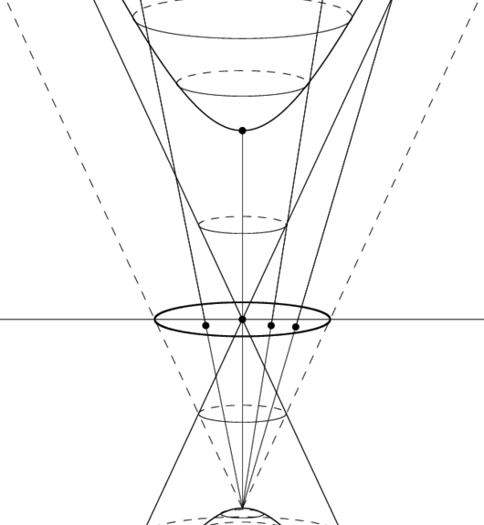
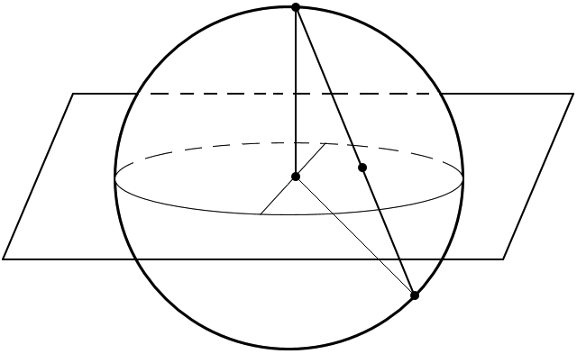
Two alternative models for hyperbolic and spherical geometries are the Poincaré ball and the stereographic projection of the sphere. Each of them result from the stereographic projection of the hyperboloid and the sphere, respectively, as illustrated in the figures below:

Hyperboloid & Poincaré Ball Sphere & Stereographic Projection of Sphere
Hyperboloid & Poincaré Ball
Sphere & Stereographic Projection of Sphere

In this blogpost we show how the duality of the Poincaré ball and the stereographic projection of the sphere can be captured within Ungar’s formalism of gyrovector spaces [5]. The reason that the stereographic projections were chosen in the model that will be presented in what follows is that they allow to smoothly interpolate between spaces of positive and spaces of negative curvature – this can be very useful to learn the curvatures of factors of product spaces used to train embeddings, but more on that in a future blogpost on curvature learning in product spaces. For now, we just want to familiarize ourselves with gyrovector spaces and our concrete instantiation of a gyrovector space: the $\kappa$-stereographic model for spherical, Euclidean and hyperbolic geometries.

Gyrovector Spaces

An important property of hyperbolic space is that it isn’t a vector space. To this end, Ungar introduced the algebraic structure of gyrovector spaces [6], which have operations and properties reminiscent of the ones of vector spaces. Indeed, gyrogroups and gyrovector spaces are a generalization of groups and vector spaces. One great advantage of gyrovector spaces is that with Ungar’s gyrovector space approach to hyperbolic geometry we get much more intuitive and concise formulas for things like geodesics, distances or the Pythagorean theorem in hyperbolic geometry.

In what follows we present the most important definitions that give rise to gyrovector spaces. The definitions presented here are taken from Ungar’s work [8], where the algebra’s axioms and and some of its deriveable properties are introduced jointly for convenience. For a presentation that restricts the definitions to a minimal set of axioms and then separately derivates the resulting properties the interested reader is referred to Ungar’s other work [5].

D. (Groupoid) A groupoid $(S, +)$ is a pair of a nonempty set $S$ and a binary operation $+\colon S\times S\to S$.
D. (Groupoid Automorphism) An automorphism $\phi$ of a groupoid $(S,+)$ is a bijective self-map of $S$ that respects its binary operation,
$$ \forall s_1,s_2\in S \colon \quad \phi(s_1 + s_2) = \phi(s_1) + \phi(s_2). $$
$$ \forall s_1,s_2\in S \colon \, \phi(s_1 + s_2) = \phi(s_1) + \phi(s_2). $$

In other words, the groupoid automorphism $\phi$ preserves the structure of the groupoid. Furthermore, the set of all automorphisms of a groupoid form a group:

D. (Automorphism Group) The set of all automorphisms of a groupoid $(S,+)$ forms a group, denoted as $\Aut(S,+)$.

Now, we define a gyrogroup, which is an essential component of a gyrovector space.

D. (Gyrogroup) A groupoid $(G,\oplus)$ is a gyrogroup if its binary operation satisfies the following axioms and properties. In $G$, there exists a unique element, $0$, called the identity, satisfying
$$ 0\oplus a= a\oplus 0= a, \qquad\text{additive identity}, $$
$$ 0\oplus a= a\oplus 0= a, $$
for all $a\in G$. For each $a$ in $G$, there exists a unique invese $\ominus a$ in $G$, satisfying
$$ \ominus a \oplus a = a\ominus a = 0,\qquad\text{inverse}, $$
$$ \ominus a \oplus a = a\ominus a = 0, $$
where we use the notation $a\ominus b=a\oplus (\ominus b)$ for $a,b\in G$. For any $a,b\in G$, the self-map $\gyr[a,b]$ of $G$ is given by the equation $$ \gyr[a,b]z = \ominus(a\oplus b) \oplus (a \oplus (b\oplus z)), $$ for all $z\in G$. Furthermore, the following conditions hold for all $a,b,c\in G$:
$$ \begin{align*} \gyr[a,b]&\in \Aut(G,\oplus), && \text{gyroautomorphism property}, \\ a\oplus (b\oplus c) &= (a \oplus b) \oplus \gyr[a,b]c, && \text{left gyroassociative law}, \\ (a\oplus b) \oplus c &= a \oplus (b \oplus \gyr[b,a]c), && \text{right gyroassociative law}, \\ \gyr[a,b] &= \gyr[a\oplus b, b], && \text{left loop property}, \\ \gyr[a,b] &= \gyr[a, b\oplus a], && \text{right loop property}, \\ \ominus(a\oplus b) &= \gyr[a,b](\ominus b\ominus a), && \text{gyrosum inversion law}, \\ \gyr^{-1}[a,b] &= \gyr[b,a], && \text{gyroautomorphism inversion}. \end{align*} $$
$$ \begin{align*} \gyr[a,b]&\in \Aut(G,\oplus), \\ a\oplus (b\oplus c) &= (a \oplus b) \oplus \gyr[a,b]c, \\ (a\oplus b) \oplus c &= a \oplus (b \oplus \gyr[b,a]c), \\ \gyr[a,b] &= \gyr[a\oplus b, b], \\ \gyr[a,b] &= \gyr[a, b\oplus a], \\ \ominus(a\oplus b) &= \gyr[a,b](\ominus b\ominus a), \\ \gyr^{-1}[a,b] &= \gyr[b,a], \end{align*} $$
The operation $\gyr\colon G\times G\to\Aut(G,\oplus)$ is called the gyrator of $G$ and the automorphism $\gyr[a,b]\colon G\to G$ is called the gyroautomorphism of $G$, generated by $a, b\in G$.

An important thing to note in the definition of the gyrogroup, is that if one was to leave out the gyrations in the definitions, one would get the properties of a group algebra. Indeed, if one instantiates the gyrogroup with vectors and vector addition, then the gyration becomes trivial and we end up with an algebra that has the properties of a group. Thus, the gyrogroup can be seen as a genralization of the group structure.

Analogously to groups and gyrogroups, the commutativity for gyrogroups is defined as fllows:

D. (Gyrocommutative Gyrogroup) A gyrogroup is gyrocommutative if it satisfies
$$ a \oplus b = \gyr[a,b](b\oplus a), \qquad \text{gyrocommutative law.} $$
$$ a \oplus b = \gyr[a,b](b\oplus a). $$

Some gyrocommutative gyrogroups admit scalar multiplication, turning them into gyrovector spaces. Just as commutative groups with a scalar multiplication give rise to vector spaces.

D. (Gyrovector Spaces) A real inner product gyrovector space $(G,\oplus,\otimes)$ (gyrovector space, in short) is a gyrocommutative gyrogroup $(G,\oplus)$ that obeys the following axioms and properties:
  1. $G$ is a subset of a real inner product vector space $\bbV$ called the carrier of $G$, $G\subseteq \bbV$, from which it inherits its inner product, $\scprod{\argdot,\argdot}$, and norm, $\norm{\argdot}$, which are invariant under gyroautomorphisms, that is,
    $$ \scprod{\gyr[\vu,\vv]\va,\gyr[\vu,\vv]\vb}=\scprod{\va,\vb}, \qquad\text{conformality}. $$
    $$ \scprod{\gyr[\vu,\vv]\va,\gyr[\vu,\vv]\vb}=\scprod{\va,\vb}. $$
  2. $G$ admits a scalar multiplication, $\otimes$, possessing the following properties. For all real numbers $r,r_1,r_2\in\R$, natural numbers $n\in\N$ and all points $\va,\vu,\vv\in G$:
    $$ \begin{align*} 1\otimes \va &= \va, && \text{multiplicative identity}, \\ n\otimes \va &= \va\oplus\cdots\oplus \va, && \text{gyroaddition }n\text{ times}, \\ (-r)\otimes\va &= r \otimes (\ominus \va), && \text{sign distributivity}, \\ (r_1+r_2)\otimes\va &= r_1\otimes \va\oplus r_2\otimes\va, &&\text{scalar distributive Law}, \\ (r_1r_2)\otimes\va &= r_1\otimes(r_2\otimes\va), &&\text{scalar associative law}, \\ r\otimes(r_1\otimes\va\oplus r_2\otimes\va) &= r\otimes(r_1\otimes\va)\oplus r\otimes(r_2\otimes\va), &&\text{monodistributive law}, \\ \frac{\abs{r}\otimes\va}{\norm{r\otimes\va}} &= \frac{\va}{\norm{\va}}, &&\text{scaling property}, \\ \gyr[\vu,\vv](r\otimes\va) &= r\otimes\gyr[\vu,\vv]\va &&\text{gyroautomorphism property}, \\ \gyr[r_1\otimes\va,r_2\otimes\va] &= \id &&\text{identity automorphism}, \\ \end{align*} $$
    $$ \begin{align*} 1\otimes \va &= \va, \\ n\otimes \va &= \va\oplus\cdots\oplus \va, \\ (-r)\otimes\va &= r \otimes (\ominus \va), \\ (r_1+r_2)\otimes\va &= r_1\otimes \va\oplus r_2\otimes\va, \\ (r_1r_2)\otimes\va &= r_1\otimes(r_2\otimes\va), \\ \frac{\abs{r}\otimes\va}{\norm{r\otimes\va}} &= \frac{\va}{\norm{\va}}, \\ \gyr[\vu,\vv](r\otimes\va) &= r\otimes\gyr[\vu,\vv]\va \\ \gyr[r_1\otimes\va,r_2\otimes\va] &= \id \end{align*} $$
    where we use the notation $r\otimes\va=\va\otimes r$.
  3. The algebra $(\norm{\G},\oplus,\otimes)$ for the set $\norm{G}$ of one-dimensional "vectors", $$ \norm{G}=\dset{\norm{\va}}{\va\in G}\subseteq\R. $$ has a real vector space structure with vector addition $\oplus$ and scalar multiplication $\otimes$, such that for all $r\in\R$ and $\va,\vb\in G$,
    $$ \begin{align*} \norm{r\otimes\va} &= \abs{r}\otimes\norm{\va}, &&\text{homogeneity property}, \\ \norm{\va\oplus\vb} &\leq \norm{\va}\oplus\norm{\vb}, &&\text{gyrotriangle property}, \end{align*} $$
    $$ \begin{align*} \norm{r\otimes\va} &= \abs{r}\otimes\norm{\va}, \\ \norm{\va\oplus\vb} &\leq \norm{\va}\oplus\norm{\vb}, \end{align*} $$
    connecting the addition and scalar multiplication of $G$ and $\norm{G}$.

From the definition of above, one can easily verify that $(-1)\otimes\va=\ominus\va$, and $\norm{\ominus\va}=\norm{\va}$. One should also note that the ambiguous use of $\oplus$ and $\otimes$ as interrelated operations in the gyrovector space $(G,\oplus,\otimes)$ and its associated one-dimensional “vector” space $(\norm{G},\oplus,\otimes)$ should not raise any confusion, since the sets in which these operations operate are always clear from the context. E.g., in vector spaces we also use the same notation, $+$, for the addition operation between vectors and between their magnitudes, and the same notation for the scalar multiplication between two scalars and between a scalar and a vector.

However, it’s important to note that the operations in the gyrovector space $(G,\oplus,\otimes)$ are nonassociative-nondistributive gyrovector space operations, and the operations in $(\norm{G},\oplus,\otimes)$ are associative-distributive vector space operations. Additionally, the gyro-addition $\oplus$ is gyrocommutative in the former, and commutative in the latter. Also note that in the vector space $(\norm{G},\oplus,\otimes)$ the gyrations are trivial.

Next, we’ll look at how we can use the algebraic structure of a gyrovector space to implement one universal model, able to capture hyperbolic, spherical and Euclidean geometries.

The $\kappa$-Stereographic Model for Hyperbolic, Spherical and Euclidean Geometry

In their paper about “Hyperbolic neural networks” [7], Ganea et al. already showed how one can harness the gyrovector space formalism presented by Ungar in [5] to implement all the necessary tools for deep neural networks that operate on hyperbolic representations. Later, throughout the development of our theses related to curvature-learning, we discovered and verified that one can use the same gyrovector space formalism also with positive sectional curvature in order to also implement all of the necessary operations for the model of the stereographic projection of the sphere.

For some $n$-dimensional manifold with constant sectional curvature $\kappa\in\R$, we can instantiate a corresponding gyrovector space algebra $(\cM_\kappa^n,\oplus_\kappa,\otimes_\kappa)$, to intuitively express and compute important operations on the manifold in closed form. The concrete definitions of the carrier set and operations for the gyrovector space algebra $(\cM_\kappa^n,\oplus_\kappa,\otimes_\kappa)$ are given in what follows.

D. (Carrier Set) The carrier set $\cM_\kappa^n$ of an $n$-dimensional gyrovector space, corresponding to a manifold of constant sectional curvature $\kappa$, is defined as: $$ \cM_\kappa^n = \dset{\vx\in\R^n}{-\kappa\norm{\vx}_2^2<1}. $$

One may easily verify that the carrier set $\cM_\kappa^n$ simplifies to the entire $\R^n$ for spherical and Euclidean geometries and to the open ball of radius $R=1/\sqrt{-\kappa}$ for hyperbolic geometries. Thus, another way to express $\cM_\kappa^n$ is:

$$ \cM_\kappa^n = \begin{cases} \dset{\vx\in\R^n}{\norm{\vx}_2<R}, & \text{for }\kappa<0, & \text{hyperbolic geometry}, \\ \R^n, & \text{for }\kappa=0, & \text{Euclidean geometry}, \\ \R^n, & \text{for }\kappa>0, & \text{spherical geometry}. \end{cases} $$
$$ \cM_\kappa^n = \begin{cases} \dset{\vx}{\norm{\vx}_2<R}, & \kappa<0, \text{ (hyp.)}, \\ \R^n, & \kappa=0, \text{ (Eucl.)}, \\ \R^n, & \kappa>0, \text{ (sph.)}. \end{cases} $$

For the addition in our gyrovector space algebra we use the plain-vanilla Möbius addition:

D. (Möbius Addition) The Möbius addition of $\vx,\vy\in\cM_\kappa^n$ is defined as
$$ \vx\oplus_\kappa\vy = \frac{ \left(1-2\kappa\scprod{\vx,\vy}-\kappa\norm{\vy}_2^2\right)\vx +\left(1+\kappa\norm{\vx}_2^2\right)\vy }{ 1 - 2\kappa\scprod{\vx,\vy}+\kappa^2\norm{\vx}_2^2\norm{\vy}_2^2 }. $$

An important property of the Möbius addition is that it recovers the Euclidean vector space addition when $\kappa\to 0$:

Having defined the Möbius addition, the Möbius subtraction is then simply defined as:

D. (Möbius Subtraction) The Möbius subtraction of $\vx,\vy\in\cM_\kappa^n$ is defined as $$ \vx\ominus_\kappa\vy = \vx\oplus_\kappa(\ominus\vy). $$

For $\kappa\leq 0$ it has been shown that $(\cM_\kappa^n,\oplus_\kappa)$ forms a commutative gyrogroup, where additive inverses are simply given as $\ominus \vx=-\vx$ [8]. Furthermore, one can easily verify that for $\kappa=0$ the gyration becomes trivial, making the algebra $(\cM_0^n,\oplus_0)$ simply a commutative group. However, it turns out that for $\kappa>0$ there are exceptions where the Möbius addition is indefinite:

T. (Definiteness of Möbius Addition) The Möbius addition is indefinite, meaning that the denominator $1-2\kappa\vx^\T\vy+\kappa^2\norm{\vx}_2^2\norm{\vy}_2^2=0$, if and only if $\kappa>0$ and $\vx=\vy/(\kappa\norm{\vy}_2^2)\neq 0$.

The theorem can be proven using the Cauchy-Schwarz inequality. Now, what this means is that for positive curvature $\kappa>0$, we have the situation that for every point $\vx$, $\vx\neq \vzero$, there exists exactly one other collinear point

for which the Möbius addition is indefinite. Therefore, strictly speaking, the gyrogroup structure is broken for $\kappa>0$ due to the indefiniteness of the Möbius addition in these cases. Hence, for $\kappa>0$ we only get a pseudo gyrogroup, which behaves like a gyrogroup, as long as the Möbius addition is definite.

However, since for every point $\vx$, $\vx\neq \vzero$, there is only exactly one other point out of the many other possible points in $\cM_\kappa^n$, for which the Möbius addition is indefinite, this is not too much of an issue for practical applications. One may circumvent these rare cases of indefinite Möbius additions by fixing them through min-clamping the denominator to a small numerical value $\epsilon>0$. This way, the Möbius addition can be extended with desirable approximation behaviour in these indefinite cases.

Before defining the scalar multiplication we first want to introduce the following trigonometric functions that are parametrized by the sectional curvature $\kappa$. These trigonometric functions will help us to unify and simplify the notations for spherical and hyperbolic geometry within the elegant formalism of gyrovector spaces.

D. (Curvature-Dependent Trigonometric Functions)
$$ \tan_\kappa(x) = \begin{cases} \frac{1}{\sqrt{-\kappa}}\tanh(\sqrt{-\kappa}x), & \kappa<0,\\ x, & \kappa=0,\\ \frac{1}{\sqrt{\kappa}}\tan(\sqrt{\kappa}x), & \kappa>0. \end{cases} $$ $$ \arctan_\kappa(x) = \begin{cases} \frac{1}{\sqrt{-\kappa}}\arctanh(\sqrt{-\kappa}x), & \kappa<0,\\ x, & \kappa=0,\\ \frac{1}{\sqrt{\kappa}}\arctan(\sqrt{\kappa}x), & \kappa>0.\\ \end{cases} $$ $$ \arcsin_\kappa(x) = \begin{cases} \frac{1}{\sqrt{-\kappa}}\arcsinh(\sqrt{-\kappa}x), & \kappa<0,\\ x, & \kappa=0,\\ \frac{1}{\sqrt{\kappa}}\arcsin(\sqrt{\kappa}x), & \kappa>0.\\ \end{cases} $$
$$ \begin{align*} &\tan_\kappa(x) = \\ &\qquad \begin{cases} \frac{1}{\sqrt{-\kappa}}\tanh(\sqrt{-\kappa}x), & \kappa<0,\\ x, & \kappa=0,\\ \frac{1}{\sqrt{\kappa}}\tan(\sqrt{\kappa}x), & \kappa>0. \end{cases} \end{align*} $$ $$ \begin{align*} &\arctan_\kappa(x) = \\ &\qquad\begin{cases} \frac{1}{\sqrt{-\kappa}}\arctanh(\sqrt{-\kappa}x), & \kappa<0,\\ x, & \kappa=0,\\ \frac{1}{\sqrt{\kappa}}\arctan(\sqrt{\kappa}x), & \kappa>0.\\ \end{cases} \end{align*} $$ $$ \begin{align*} &\arcsin_\kappa(x) = \\ &\qquad\begin{cases} \frac{1}{\sqrt{-\kappa}}\arcsinh(\sqrt{-\kappa}x), & \kappa<0,\\ x, & \kappa=0,\\ \frac{1}{\sqrt{\kappa}}\arcsin(\sqrt{\kappa}x), & \kappa>0.\\ \end{cases} \end{align*} $$

If one ignores the definitions of the upper functions for the cases where $\kappa=0$, one may verify that for any $f_\kappa\in\set{\tan_\kappa,\arctan_\kappa,\arcsin_\kappa}$ the identity map is approached as $\kappa\to 0$:

This is exactly the motivation behind the definitions of the cases where $\kappa=0$. Also, these limits will become useful later when we’ll show how the $\kappa$-stereographic model approaches an Euclidean geometry for $\kappa\to 0$.

Having defined these curvature-dependent trigonometric functions we can now use them to define an augmented version of the Möbius scalar multiplication as follows:

D. (Augmented Möbius Scalar Multiplication) The augmented Möbius scalar multiplication of $\vx\in\cM_\kappa^n\setminus\set{\vo}$ by $\alpha\in\R$ is defined as $$ \alpha\otimes_\kappa \vx = \tan_\kappa \left( \alpha \arctan_\kappa \left( \norm{\vx}_2 \right)\right) \frac{\vx}{\norm{\vx}_2}. $$

Hence, the augmented Möbius scalar multiplication only distinguishes itself from the conventional Möbius scalar multiplication through the usage of our parametrized trigonometric functions that also support nonnegative curvature $\kappa\geq0$. However, there’s one subtlety for $\kappa > 0$ that has to be considered:

T. (Definiteness of Augmented Möbius Scalar Multiplication) The augmented Möbius scalar multiplication is indefinite, if and only if $\kappa>0$ and $\alpha\arctan_{\kappa}(\norm{\vx}_2)=\frac{\pi}{2}+k\pi$ for some $k\in\Z$.

However, this indefiniteness is not too tragic. One may redefine the augmented scalar multiplication for an indefinite case $\alpha\otimes_k\vx$ recursively as

giving an augmented gyrovector scalar multiplication that is definite for all real scalars.

Having defined the carrier set, the gyrovector space addition and the scalar multiplication we now have everything for our (pseudo) gyrovector space algebra $(\cM_\kappa^n,\oplus_\kappa,\otimes_\kappa)$. Now, let’s have a look at how we can use this (pseudo) gyrovector space algebra to express all the necessary operations for the Poincaré ball ($\kappa<0$) and the stereographic projection of the sphere ($\kappa>0$):

Description Closed-Form Formula on $\cM_\kappa^n$, $\kappa\neq 0$
Radius $R:=\frac{1}{\sqrt{\abs{\kappa}}}\in(0,\infty)$
Tangent Space $\cT_{\vx}\cM_\kappa^n=\bbR^n$
Conformal Factor $ \lambda_{\vx}^\kappa = \frac{2}{1+\kappa\norm{\vx}_2^2} \in (0,\infty) $
Metric Tensor $ \vg^{\kappa}_{\vx} = \left(\lambda_{\vx}^\kappa\right)^2\MI \in \R^{n\times n} $
Tangent Space Inner Product
$\scprod{\argdot,\argdot}_{\vx}^\kappa\colon\cT_{\vx}\cM_\kappa^n\times\cT_{\vx}\cM_\kappa^n\to\R$
$ \scprod{\vu,\vv}_{\vx}^\kappa = \vu^T\vg_{\vx}^\kappa\vv = (\lambda_{\vx}^\kappa)^2\scprod{\vu,\vv}$
Tangent Space Norm
$\norm{\argdot}_{\vx}^\kappa\colon\cT_{\vx}\cM_\kappa^n\to\R^+_0$
$\norm{\vu}_{\vx}^\kappa=\lambda_{\vx}^\kappa\norm{\vu}_2$
Angle $\theta_{\vx}(\vu,\vv)$ between two Tangent Vectors $\vu,\vv\in\cT_{\vx}\cM_\kappa^n\setminus\set{\vo}$ $ \theta_{\vx}(\vu,\vv) =\arccos\left( \frac{\scprod{\vu,\vv}}{\norm{\vu}_2\norm{\vv}_2} \right) \quad\text{(conformal)} $
Distance
$d_{\kappa}\colon \cM_\kappa^n\times \cM_\kappa^n\to\R^+_0$
$ d_{\kappa}(\vx,\vy) = 2\arctan_\kappa\left(\norm{(-\vx)\oplus_\kappa\vy}_2\right) $
Distance of $\vx$ to Hyperplane $H_{\vp,\vw}$ Described by Point $\vp$ and Normal Vector $\vw$
$d_{\kappa}^{H_{\vp,\vw}}\colon \cM_\kappa^n\to\R^+_0$
$ d_\kappa^{H_{\vp,\vw}}(\vx) = \arcsin_\kappa\left( \frac{ 2 \abs{\scprod{-\vp)\oplus_\kappa \vx, \vw}} }{ \left(1+\kappa\norm{(-\vp)\oplus_\kappa \vx}_2^2\right)\norm{\vw}_2 } \right) $
Exponential Map
$\exp_{\vx}^{\kappa}\colon\cT_{\vx}\cM_\kappa^n\to\cM_\kappa^n$
$ \exp_{\vx}^{\kappa}(\vu) = \vx\oplus_\kappa \left( \tan_\kappa\left( \frac{1}{2} \norm{\vu}_{\vx}^\kappa \right) \frac{\vu}{\norm{\vu}_2} \right) $
Log Map
$\log_{\vx}^\kappa\colon\cM_\kappa^n\to\cT_{\vx}\cM_\kappa^n$
$ \log_{\vx}^\kappa(\vy)= 2\arctan_\kappa\left(\norm{(-\vx)\oplus_\kappa\vy}_2\right) \frac{(-\vx)\oplus_\kappa \vy}{\norm{(-\vx)\oplus_\kappa \vy}_{\vx}^\kappa} $
$ \begin{align*} &\log_{\vx}^\kappa(\vy)= \\ &\quad 2\arctan_\kappa\left(\norm{(-\vx)\oplus_\kappa\vy}_2\right) \frac{(-\vx)\oplus_\kappa \vy}{\norm{(-\vx)\oplus_\kappa \vy}_{\vx}^\kappa} \end{align*} $
Geodesic from $\vx\in\cM_\kappa^n \text{ to } \vy\in\cM_\kappa^n$
$\vgamma_{\vx\to\vy}^\kappa\colon [0,1]\to\cM_\kappa^n$
$ \vgamma_{\vx\to\vy}^{\kappa}(t)=\vx\oplus_\kappa\left(t\otimes_\kappa\left((-\vx) \oplus_\kappa\vy\right) \right) $
Unit-Speed Geodesic at Time $t\in\R$ Starting from $\vx\in\cM_\kappa^n$ in Direction of $\vu\in\cT_{\vx}\cM_\kappa^n$
$\vgamma_{\vx,\vu}^{\kappa}\colon \R\to\cM_\kappa^n$
$ \vgamma_{\vx,\vu}^{\kappa}(t) = \vx \oplus_\kappa \left( \tan_\kappa\left( \frac{1}{2}t \right) \frac{\vu}{\norm{\vu}_2} \right) $
Antipode $\vx^a$ of $\vx$ for $\kappa>0$ $ \vx^a = \frac{1}{\lambda_{\vx}^{\kappa}\kappa\norm{\vx}_2^2}(-\vx) $
Weighted Midpoint
$\vm_{\kappa}\colon (\cM_\kappa^d)^n\times\R^n\to\cM_\kappa^d$
$ \vm_\kappa(\vx_{1:n},\alpha_{1:n}) = \frac{1}{2} \otimes_\kappa \left( \sum_{i=1}^n \frac{ \alpha_i\lambda_{\vx_i}^\kappa }{ \sum_{j=1}^n\alpha_j(\lambda_{\vx_i}^\kappa - 1) } \vx_i \right) $
$ \begin{align*} &\vm_\kappa(\vx_{1:n},\alpha_{1:n}) =\\ &\quad \frac{1}{2} \otimes_\kappa \left( \sum_{i=1}^n \frac{ \alpha_i\lambda_{\vx_i}^\kappa }{ \sum_{j=1}^n\alpha_j(\lambda_{\vx_i}^\kappa - 1) } \vx_i \right) \end{align*} $
for $\kappa>0$ this also requires determining which of $\vm_{\kappa}$ and $\vm_{\kappa}^a$ minimizes the sum of distances

The formulas in the table above clearly illustrate how dual the Poincaré ball and the stereographic projection of the sphere are. In hindsight, the duality of the two stereographic models is not so surpising, since both models are the stereographic projections of the hyperboloid and the sphere, which are known to be dual. Now, let’s see next how the dual models connect even more for $\kappa\to 0$.

Recovery of Euclidean Geometry as $\kappa\to 0$

The following formulas show how in the limit $\kappa\to\ 0$ an Euclidean geometry, with a Cartesian coordinate system at intervals of $2$ units, is recovered:

Description Closed-Form Formula on $\cM_\kappa^n$ for $\kappa\to 0$
Radius $R\to\infty$
Tangent Space $\cT_{\vx}\cM_0^n=\bbR^n$
Conformal Factor $ \lambda_{\vx}^0 = 2 $
Metric Tensor $ \vg^{0}_{\vx} = (\lambda_{\vx}^0)^2\MI = 4\MI \in \R^{n\times n} $
Tangent Space Inner Product
$\scprod{\argdot,\argdot}_{\vx}^0\colon\cT_{\vx}\cM_0^n\times\cT_{\vx}\cM_0^n\to\R$
$ \scprod{\vu,\vv}_{\vx}^0 = \vu^T\vg_{\vx}^0\vv = (\lambda_{\vx}^0)^2\scprod{\vu,\vv} = 4\scprod{\vu,\vv} $
Tangent Space Norm
$\norm{\argdot}_{\vx}^0\colon\cT_{\vx}\cM_0^n\to\R^+_0$
$\norm{\vu}_{\vx}^0=\lambda_{\vx}^0\norm{\vu}_2=2\norm{\vu}_2$
Angle $\theta_{\vx}(\vu,\vv)$ between two Tangent Vectors $\vu,\vv\in\cT_{\vx}\cM_0^n\setminus\set{\vo}$ $ \theta_{\vx}(\vu,\vv) =\arccos\left( \frac{\scprod{\vu,\vv}}{\norm{\vu}_2\norm{\vv}_2} \right) $
Distance
$d_{0}\colon \cM_0^n\times \cM_0^n\to\R^+_0$
$ d_{0}(\vx,\vy) = 2\norm{\vx-\vy}_2 $
Distance of $\vx$ to Hyperplane $H_{\vp,\vw}$ Described by Point $\vp$ and Normal Vector $\vw$
$d_{\kappa}^{H_{\vp,\vw}}\colon \cM_\kappa^n\to\R^+_0$
$ d_\kappa^{H_{\vp,\vw}}(\vx) = 2 \abs{\scprod{\vx-\vp, \frac{\vw}{\norm{\vw}_2} }} $
Exponential Map
$\exp_{\vx}^{0}\colon\cT_{\vx}\cM_0^n\to\cM_0^n$
$ \exp_{\vx}^{0}(\vu) = \vx+\vu $
Log Map
$\log_{\vx}^0\colon\cM_0^n\to\cT_{\vx}\cM_0^n$
$ \log_{\vx}^0(\vy)= \vy-\vx $
Geodesic from $\vx\in\cM_0^n \text{ to } \vy\in\cM_0^n$
$\vgamma_{\vx\to\vy}^0\colon [0,1]\to\cM_0^n$
$ \vgamma_{\vx\to\vy}^{0}(t) = \vx+t(\vy-\vx) $
Unit-Speed Geodesic at Time $t\in\R$ Starting from $\vx\in\cM_0^n$ in Direction of $\vu\in\cT_{\vx}\cM_0^n$
$\vgamma_{\vx,\vu}^{0}\colon \R\to\cM_0^n$
$ \vgamma_{\vx,\vu}^{0}(t) = \vx + \frac{1}{2}t \frac{\vu}{\norm{\vu}_2} $
Weighted Midpoint
$\vm_{0}\colon (\cM_\kappa^d)^n\times\R^n\to\cM_\kappa^d$
$ \vm_\kappa(\vx_{1:n},\alpha_{1:n}) = \sum_{i=1}^n \frac{ \alpha_i }{ \sum_{j=1}^n\alpha_j } \vx_i $

The formulas for the Euclidean geometry have a “2” or a “4” here and there which comes from the fact that the points $\vx,\vy$ are in the basis of a Cartesian coordinate system with intervals of size 2. This coordinate system just emerges in the limit $\kappa\to 0$ from the Poincaré ball and also from the stereographic projection of the sphere, which both can be seen as a coordinate systems for a corresponding hyperbolic and spherical geometry, respectively.

A few things to note in the formulas of above are: that the exponential- and the logmap are simply given through vector addition and subtraction. Also, the distance is simply upscaled by a factor of 2 due to the choice of coordinates. The weighted midpoint simply becomes the familiar weighted average.

Grids of Geodesics at Equidistant Intervals

Now that we’ve entirely described the models mathematically, let’s also build up our intuitions through some illustrations of the geometries in 2D. First, we want to see how a grid of equidistant geodesics in two orthogonal directions looks like in the geometries of constant curvature.

Grid of Geodesics on Euclidean Manifold

Here’s how a grid of geodesics looks like on the $x/y$-plane, a.k.a. the 2D Euclidean manifold. Actually, that’s nothing special, the grid just consists of straight lines, reminding us of the Cartesian coordinate system. Note that this 2D grid could be a cross-section of a 3D Euclidean geometry.

Grid of Geodesics at Equidistant Intervals
on Euclidean Manifold
($\kappa=0$)
Grid of Geodesics at Equidistant Intervals on Euclidean Manifold

Grid of Geodesics on Poincaré Ball

Now, let’s get a feeling of how a grid of geodesics at equidistant intervals on the $x/y$-axes looks like on the Poincaré disk:

Grid of Geodesics at Equidistant Intervals
on Poincaré Ball
($\kappa=-1$)
Grid of Geodesics at Equidistant Intervals on Poincaré Ball

Recall, that the points on the Poincaré disk result from the stereographic projection of the hyperboloid. Here are a few things to note about the grid of geodesics on the Poincaré ball.

  • The center of the Poincaré ball, which we also refer to as the origin, represents the lower tip of the upper sheet of the two-sheeted hyperboloid.
  • The border of the Poincaré ball represents points at infinity, or alternatively, points on the hyperboloid that are infinitely far away from the origin.
  • The geodesics intersect the border of the Poincaré ball at a right angle.
  • From a plain "eye" point-of-view the interval between the geodesics becomes tighter and tighter towards the border of the Poincaré ball. But according to the hyperbolic metric they are equidistant. This tightening happens because volumes and distances towards border of the Poincaré ball grow exponentially, since close to the border, even small dislocations on the Poincaré ball correspond to large dislocations on the hyperboloid.

One can also imagine how a 3D hyperbolic geometry looks like if one imagines that this 2D grid of geodesics is the cross-section of the inside of a 3D Poincaré ball.

Grid of Geodesics on Stereographic Projection of Sphere

Here’s how the equivalent grid of geodesics looks like for the stereographic projection of the 2D sphere:

Grid of Geodesics at Equidistant Intervals
on Stereographic Projection of Sphere
($\kappa=1$)
Grid of Geodesics at Equidistant Intervals on Stereographic Projection of Sphere

Some things to note in this grid are:

  • The center inside the ball is the stereographic projection of the south pole.
  • The ball marked in bold corresponds to the equator of the 2D sphere.
  • All the geodesics actually represent a great-circle of the 2D sphere.
  • The geodesic length of the part of a great-circle that is inside the bold ball (equator) is equal to the geodesic length of the part of the great-circle that is on the outside of the equator.
  • Each pair of geodesics meets exactly twice.

Similarly, one can also imagine how a 3D spherical geometry would look like if one thinks of this grid as a cross-section of a 3D spherical geometry.

Illustrations of Smooth Interpolations between Geometries of Positive and Negative Curvature

In the following we want to illustrate how the $\kappa$-stereographic model allows to compute useful notions for the manifolds of constant curvature and how these notions smoothly interpolate for changes of the curvature $\kappa$.

Parallel Transport of Unit Gyrovectors

The following animation shows how the parallel transport of unit gyrovectors smoothly adapts to changing values of the curvature $\kappa$:

Parallel Transport of Gyrovectors

Midpoints

The following animation shows how the equally-weighted geodesic midpoint $\vm_{\kappa}$ of $\vx_1,\ldots,\vx_4$ smoothly changes for changes in $\kappa$. The corresponding shortest paths from the points $\vx_1,\ldots,\vx_4$ to their midpoint $\vm_{\kappa}$ are also illustrated. For positive curvature the antipode of the midpoint $\vm_{\kappa}$ is also shown.

Midpoint
Midpoint

Observe how for positive curvature the midpoint moves to the northern hemisphere once that the embeddings of $\vx_1,\ldots,\vx_4$ also start to reside there.

Geodesic Distance

The following animation shows how the scalar field of distances to a point $\vx$ smoothly transforms for various curvatures. One thing to note here is how for spherical geometries with a large curvature the maximal representable distance becomes very small due to the spherical structure of the manifold. Another thing to notice for negative curvature is that most of the space resides at the border of the Poincaré ball - thus it is crucial to work with float64 in order to represent distances accurately.

Geodesic Distance
Distance
Heatmap of square root of distance $\sqrt{d_{\kappa}(\vx,\argdot)}$ to $\vx$

Hyperplane Distance

The following animation shows how the scalar field of distances to a hyperplane smoothly transforms for various curvatures. The hyperplane is described by a a point $\vp$ on the hyperplane and a normal vector $\vw$. Note how the hyperplane just becomes a straight line for $\kappa\to 0$ and a great-cricle for $\kappa>0$:

Hyperplane Distance
Distance to Hyperplane
Heatmap of square root of hyperplane distance $\sqrt{d_{\kappa}^{H_{\vp,\vw}}(\argdot)}$

Implementation of $\kappa$-Stereographic Model

An Pytorch implementation of the $\kappa$-stereographic model was contributed by Andreas Bloch to the open-source geometric optimization library geoopt. The code for the $\kappa$-stereographic model can be found here:

$\kappa$-Stereographic Model Source

Note that the implementation doesn’t support the Euclidean geometry for $\kappa=0$. Instead only the cases $\abs{\kappa}>0.001$ are supported, such that the formulas of above always provide gradients for $\kappa$ in order to be able to learn the curvatures of embedding spaces.

Code Example for $\kappa$-Stereographic Model

Here’s a quick code example that shows how the $\kappa$-stereographic model can be instantiated and used to perform some of the aforementioned operations. The code example also shows how to train the curvature $\kappa$ to achieve certain targets.

import torch
from geoopt.manifolds.stereographic import StereographicExact
from geoopt.optim import RiemannianAdam
from geoopt import ManifoldTensor
from geoopt import ManifoldParameter

# MANIFOLD INSTANTIATION AND COMPUTATION OF MANIFOLD QUANTITIES ################


# create manifold with initial K=-1.0 (Poincaré Ball)

manifold = StereographicExact(K=-1.0,
                              float_precision=torch.float64,
                              keep_sign_fixed=False,
                              min_abs_K=0.001)

# get manifold properties

K = manifold.get_K().item()
R = manifold.get_R().item()
print(f"K={K}")
print(f"R={R}")

# define dimensionality of space

n = 10

def create_random_point(manifold, n):
    x = torch.randn(n)
    x_norm = x.norm(p=2)
    x = x/x_norm * manifold.get_R() * 0.9 * torch.rand(1)
    return x

# create two random points on manifold

x = create_random_point(manifold, n)
y = create_random_point(manifold, n)

# compute their initial distances

initial_dist = manifold.dist(x, y)
print(f"initial_dist={initial_dist.item():.3f}")

# compute the log map of y at x

v = manifold.logmap(x, y)

# compute tangent space norm of v at x (should be equal to initial distance)

v_norm = manifold.norm(x, v)
print(f"v_norm={v_norm.item():.3f}")

# compute the exponential map of v at x (=y)

y2 = manifold.expmap(x, v)
diff = (y-y2).abs().sum()
print(f"diff={diff.item():.3f}")

# CURVATURE OPTIMIZATION #######################################################


# define embedding_optimizer for curvature

curvature_optimizer = torch.optim.SGD([manifold.get_trainable_K()], lr=1e-2)

# set curvature to trainable

manifold.set_K_trainable(True)

# define training loop to optimize curvature until the points have a

# certain target distance

def train_curvature(target_dist):
    for t in range(100):
        curvature_optimizer.zero_grad()
        dist_now = manifold.dist(x,y)
        loss = (dist_now - target_dist).pow(2)
        loss.backward()
        curvature_optimizer.step()

# keep the points x and y fixed,

# train the curvature until the distance is 0.1 more than the initial distance

# --> curvature smaller than initial curvature

train_curvature(initial_dist + 1.0)
print(f"K_smaller={manifold.get_K().item():.3f}")

# keep the points x and y fixed,

# train the curvature until the distance is 0.1 less than the initial distance

# --> curvature greater than initial curvature

train_curvature(initial_dist - 1.0)
print(f"K_larger={manifold.get_K().item():.3f}")

# EMBEDDING OPTIMIZATION #######################################################


# redefine x and y as manifold parameters and assign them to manifold such

# that the embedding_optimizer knows according to which manifold the gradient

# steps have to be performed

x = ManifoldTensor(x, manifold=manifold)
x = ManifoldParameter(x)
y = ManifoldTensor(y, manifold=manifold)
y = ManifoldParameter(y)

# define embedding optimizer and pass embedding parameters

embedding_optimizer = RiemannianAdam([x, y], lr=1e-1)

# define a training loop to optimize the embeddings of x and y

# until they have a certain distance

def train_embeddings(target_dist, x, y):
    for t in range(1000):
        embedding_optimizer.zero_grad()
        dist_now = manifold.dist(x,y)
        loss = (dist_now - target_dist).pow(2)
        loss.backward()
        embedding_optimizer.step()

# print current distance

print(f"dist(x,y)={manifold.dist(x,y).item():.3f}")

# optimize until points have target distance of 4.0

train_embeddings(4.0, x, y)
print(f"dist(x,y)={manifold.dist(x,y).item():.3f}  target:4.0")

# optimize until points have target distance of 2.0

train_embeddings(2.0, x, y)
print(f"dist(x,y)={manifold.dist(x,y).item():.3f}  target:2.0")

That’s all for the $\kappa$-stereographic model. We hope that this blogpost and the provided implementation supports the sparking of new ideas for applications of our $\kappa$-stereographic model.

References

  1. A. Gu, F. Sala, B. Gunel, and C. Ré, “Learning Mixed-Curvature Representations in Product Spaces,” 2018.
  2. O. Skopek, O.-E. Ganea, and G. Bécigneul, “Mixed-curvature Variational Autoencoders,” arXiv preprint arXiv:1911.08411, 2019.
  3. G. Bachmann, G. Bécigneul, and O.-E. Ganea, “Constant Curvature Graph Convolutional Networks,” arXiv preprint arXiv:1911.05076, 2019.
  4. R. C. Wilson, E. R. Hancock, E. Pekalska, and R. P. W. Duin, “Spherical and hyperbolic embeddings of data,” IEEE transactions on pattern analysis and machine intelligence, vol. 36, no. 11, pp. 2255–2269, 2014.
  5. A. A. Ungar, Analytic hyperbolic geometry: Mathematical foundations and applications. World Scientific, 2005.
  6. A. A. Ungar, “Thomas precession and its associated grouplike structure,” American Journal of Physics, vol. 59, no. 9, pp. 824–834, 1991.
  7. O. Ganea, G. Bécigneul, and T. Hofmann, “Hyperbolic neural networks,” in Advances in neural information processing systems, 2018, pp. 5345–5355.
  8. A. A. Ungar, “Hyperbolic trigonometry and its application in the Poincaré ball model of hyperbolic geometry,” Computers & Mathematics with Applications, vol. 41, no. 1-2, pp. 135–147, 2001.