Stochastic Gradient Descent on Riemannian Manifolds

In this blogpost I’ll explain how Stochastic Gradient Descent (SGD) is generalized to the optimization of loss functions on Riemannian manifolds. First, I’ll give an overview of the kind of problems that are suited for Riemannian optimization. Then, I’ll explain how Riemannian Stochastic Gradient Descent (RSGD) works in detail and I’ll also show how RSGD is performed in the case where the Riemannian manifold of interest is a product space of several Riemannian manifolds. If you’re already experienced with SGD and you’re just about getting started with Riemannian optimization this blogpost is exactly what you were looking for.

Typical Riemannian Optimization Problems

Let’s first consider the properties of optimization problems that we’d typically want to solve through Riemannian optimization. Riemannian optimization is particularly well-suited for problems where we want to optimize a loss function

that is defined on a Riemannian manifold $(\cM,g)$. This means that the optimization problem requires that the optimized parameters $\vtheta\in\cM$ lie on the “smooth surface” of a Riemannian manifold $(\cM,g)$. One can easily think of constrained optimization problems where the constraint can be described through points lying on a Riemannian manifold (e.g., the parameters must lie on a sphere, the parameters must be a rotation matrix, …). Riemannian optimization then gives us the possibilty of turning a constrained optimization problem into an unconstrained one that can be naturally solved via Riemannian optimization.

So, in Riemannian optimization we’re interested in finding an optimal solution $\vtheta^*$ for our parameters

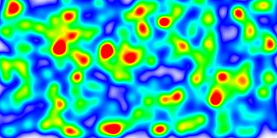
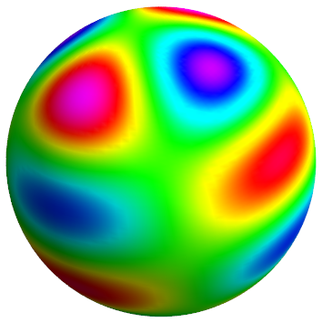
that lie on a Riemannian manifold. The following two figures illustrate the heatmaps of some non-convex loss functions, that are defined on an Euclidean and spherical Riemannian manifold.

Heatmap of a loss function $\cL$ defined on the Euclidean plane

Heatmap of a loss function $\cL$ defined on a spherical manifold

Similarly as with SGD in Euclidean vector spaces, in Riemannian optimization we want to perform a gradient-based descent on the surface of the manifold. The gradient steps should also be based on the gradients of the loss fuction $\cL$, such that we finally find some parameters $\vtheta^*$ that hopefully lie at a global minimum of the loss.

What’s Different with SGD on Riemannian Manifolds?

Let’s first look at what makes RSGD different from the usual SGD in the Euclidean vector spaces. Actually, RSGD just works like SGD when applied to our well-known Euclidean vector spaces, because RSGD is just a generalization of SGD to arbitrary Riemannian manifolds.

Indeed, the Euclidean vector space $\R^n$ can be interpreted as a Riemannian manifold $(\R^n, g_{ij})$, known as the Euclidean manifold, with the metric $g_{ij}=\delta_{ij}$. When using our usual SGD to optimize a loss function defined over the Euclidean manifold $\R^n$, we iteratively compute the following gradients and gradient updates on minibatches in order to hopefully converge to an optimal solution:

Now, in some optimization problems the solution space, or solution manifold $\cM$, might have a structure that is different from the Euclidean manifold. Let’s consider two examples of optimization problems that can be captured as Riemannian optimization problems and let’s have a look at the challenges that arise in the gradient updates:

1. Points on a Sphere: The optimization problem may require that the parameters $\vtheta=(x,y,z)$ lie on a 2D-spherical manifold of radius 1 that is embedded in 3D ambient space. The corresponding Riemannian manifold $(\cM,g)$ would then be

   $$\begin{align*} \cM&=\sdset{\vtheta\in\R^{3}}{\norm{\vtheta}_2=1}, \\ g&=\MI. \end{align*}$$

   In this case we have a loss function $\cL\colon\cM\to\R$ that gives us the loss for any point (or parameter) $\vtheta$ on the sphere $\cM$. Our machine learning framework might then automatically provide us with the derivatives of the loss

   $$ \vh(\vtheta^{(t)}) = \left( \fpartial{\cL(\vtheta^{(t)})}{x}, \fpartial{\cL(\vtheta^{(t)})}{y}, \fpartial{\cL(\vtheta^{(t)})}{z} \right) $$
   $$ \vh(\vtheta^{(t)}) = \left( \tfrac{\partial\cL(\vtheta^{(t)})}{\partial x}, \tfrac{\partial\cL(\vtheta^{(t)})}{\partial y}, \tfrac{\partial\cL(\vtheta^{(t)})}{\partial z} \right) $$

   evaluated at our current parameters $\vtheta^{(t)}$. But now, how are we going about updating the parameters $\vtheta^{(t)}$ with $\vh(\vtheta^{(t)})$? We can’t just use our well-known update-rule of SGD for Euclidean vector spaces, since we’re not guaranteed that the update rule

   $$\vtheta^{(t+1)}\gets\vtheta^{(t)}-\eta_t\vh(\vtheta^{(t)})$$

   yields a valid update $\vtheta^{(t+1)}$ that lies on the surface of spherical manifold $\cM$. Before seeing how this can be solved through Riemannian optimization, let’s first consider another example where we encounter a similar issue.

2. Doubly-Stochastic Matrices: One may also think of a more complicated optimization problem, where the parameters $\vtheta$ must be a square matrix with positive coefficients such that the coefficients of every row and column sum up to 1. It turns out that this solution space $\cM$ also represents a Riemannian manifold, having thus a smooth “surface” and a metric $g_{\MX}$ that smoothly varies with $\MX$. This Riemannian manifold $(\cM,g_{\MX})$ is the manifold of so-called doubly-stochastic matrices [1], given by:

   $$ \begin{align*} \cM&=\dset{\MX\in\R^{d\times d}}{ \begin{array}{rl} \forall i,j\in\set{1,\ldots,d}\colon &X_{ij}\geq 0, \\ \forall i\in\set{1,\ldots,d}\colon &\sum_{k=1}^d X_{ik}=\sum_{k=1}^d X_{ki} = 1. \end{array} }, \\ g_{\MX}&=\Tr{(\MA\oslash\MX)\MB^\T}. \end{align*} $$
   $$ \cM=\dset{\MX\in\R^{d\times d}}{ \begin{array}{c} \forall i,j\in\set{1,\ldots,d}\colon \\ X_{ij}\geq 0, \\ \sum_{k=1}^d X_{ik}=1, \\ \sum_{k=1}^d X_{ki}=1. \end{array} }, $$ $$ g_{\MX}=\Tr{(\MA\oslash\MX)\MB^\T}. $$

   Again, our machine learning framework may give us the derivatives of the loss w.r.t. each of the parameter matrix’ coefficients and evaluate it at our current parameters $\vtheta^{(t)}:$

   $$\MH(\vtheta^{(t)}) = \left( \fpartial{\cL(\vtheta)}{X_{ij}} \right)_{i,j=1}^{d}.$$

   Again, the simple gradient-update rule of SGD for parameters in Euclidean vector spaces

   $$\vtheta^{(t+1)}\gets\vtheta^{(t)}-\eta_t\MH(\vtheta^{(t)})$$

   would not guarantee us that the update always yields a matrix $\vtheta^{(t+1)}$ with nonnegative coefficients whose rows and columns sum up to 1.

In both examples we saw that the simple SGD update-rule for Euclidean vector spaces is insufficient to guarantee the validity of the updated parameters. So now the question is, how can we perform valid gradient updates to parameters that are defined on arbitrary Riemannian manifolds? – That’s exactly where Riemannian optimization comes in, which we’ll look at next!

Performing Gradient Steps on Riemannian Manifolds

In the “curved” spaces of Riemannian manifolds the gradient updates ideally should follow the “curved” geodesics instead of just following straight lines as done in SGD for parameters on our familiar Euclidean manifold $\bbR^n$. To this end, the seminal work of Bonnabel [2] introduced Riemannian Stochastic Gradient Descent (RSGD) that generalizes SGD to Riemannian manifolds. In what follows I’ll explain and illustrate how this technique works.

Let’s now assume that we have a typical Riemannian optimization problem, e.g., one of the two mentioned previously, where the solution space is given by an arbitrary $d$-dimensional Riemannian manifold $(\cM, g)$ and we’re interested in finding an optimal solution of a loss function $\cL\colon\cM\to\cR$, that is defined for any parameters $\vtheta$ on the Riemannian manifold. Let $\vtheta^{(t)}\in\cM$ denote our current set of parameters at timestep $t$. A gradient-step is then performed through the application of the following three steps:

1. Evaluate the gradient of $\cL$ w.r.t. the parameters $\vtheta$ at $\vtheta^{(t)}$.

2. Orthogonally project the gradient onto the tangent space $\cT_{\vtheta^{(t)}}\cM$ to get the tangent vector $\vv$, pointing in the direction of steepest ascent of $\cL$.

3. Perform a gradient-step on the surface of the manifold in the negative direction of the tangent vector $\vv$, to get the updated parameters.

We’ll now look at these steps in more detail in what follows.

Computation of Gradient w.r.t. Current Parameters

In order to minimize our loss function $\cL$, we first have to determine the gradient. The gradient w.r.t. our parameters $\vtheta$, evaluated at our current parameters $\vtheta^{(t)}$, is computed as follows:

The computation and evaluation of the derivatives $\fpartial{\cL(\vtheta^{(t)})}{\vtheta}$ is usually just performed automatically through the auto-differentiation functionality of our machine learning framework of choice. However, the multiplication with the inverse metric $\vg^{-1}_{\vtheta^{(t)}}$ usually has to be done manually in order to obtain the correct quantity for the gradient $\nabla_{\vtheta}\cL(\vtheta^{(t)})$.

If that should be new to you that we have to multiply the partial derivatives by the inverse of the metric tensor $\vg^{-1}_{\vtheta^{(t)}}$ to obtain the gradient then don’t worry too much about that now. Let me just tell you that, actually, that’s how the gradient is defined in general. The reason you might have never come across this multiplication by the inverse metric tensor is that for the usual Euclidean vector space, with the usual Cartesian coordinate system, the inverse metric tensor $\vg^{-1}$ just simplifies to the identity matrix $\MI$, and is therefore usually omitted for convenience.

The reason behind the multiplication by the inverse metric tensor is that we want the gradient to be a vector that is invariant under the choice of a specific coordinate system. Furthermore, it should satisfy the following two properties that we already know from the gradient in Euclidean vector spaces:

• The gradient evaluated at $\vtheta^{(t)}$ points into the direction of steepest ascent of $\cL$ at $\vtheta^{(t)}$.

• The norm of the gradient at $\vtheta^{(t)}$ is equal to the value of the directional derivative in a unit vector of the gradient’s direction.

Explaining the reasons behind the multiplication with $\vg^{-1}_{\vtheta^{(t)}}$ in more detail would explode the scope of this blogbost. However, in case you should want to learn more about this, I highly recommend that you have a look at Pavel Grinfield’s valuable lectures on tensor calculus (until Lesson 5a for the gradient), where you can learn the reasons behind the multiplication with the inverse metric tensor in a matter of a few hours.

Orthogonal Projection of Gradient onto Tangent Space

Since the previously computed gradient $\vh=\nabla_{\vtheta}\cL(\vtheta^{(t)})$ may be lying just somewhere in ambient space, we first have to determine the component of $\vh$ that lies in the tangent space at $\vtheta^{(t)}$. The situation is illustrated in the figure below, where we can see our manifold $\cM$, the gradient $\vh$ lying in the ambient space, and the tangent space $\cT_{\vtheta^{(t)}}\cM$, which represents a first-order approximation of the manifold’s surface around our current parameters $\vtheta^{(t)}$.

Orthogonal Projection of Gradient $\vh=\nabla_{\vtheta}\cL(\vtheta^{(t)})$ onto Tangent Space $\cT_{\vtheta^{(t)}}\cM$

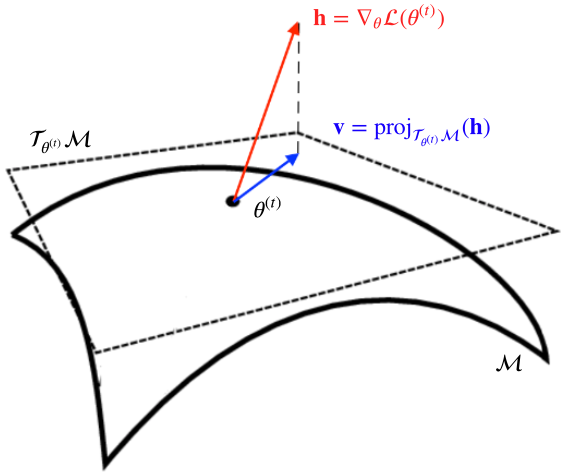
The component of $\vh$ that lies in $\cT_{\vtheta^{(t)}}\cM$ is determined through the orthogonal projection of $\vh$ from the ambient space onto the tangent space $\cT_{\vtheta^{(t)}}\cM$:

Depending on the chosen representation for the manifold $\cM$ it might even be that the orthogonal projection is not even necessary, e.g., in the case where any tangent space is always equal to the ambient space.

Gradient Step from Tangent Vector

Having determined the direction of steepest increase $\vv$ of $\cL$ in the tangent space $\cT_{\vtheta^{(t)}}\cM$ we can now use it to perform a gradient step. As with the usual SGD, we want to take a step in the negative gradient direction in order to hopefully decrease the loss. Thus, in the tangent space, we take a step in the direction of $-\eta_t\vv$, where $\eta_t$ is our learning rate, and obtain the point $-\eta_t\vv$ in the tangent space $\cT_{\vtheta^{(t)}}$.

Recall, that the tangent space $\cT_{\vtheta^{(t)}}$ represents a first-order approximation of the manifold’s smooth surface at the point $\vtheta^{(t)}$. Hence, the vector $-\eta_t\vv\in\cT_{\vtheta^{(t)}}$ is in a direct correspondence with the point $\vtheta^{(t+1)}\in\cM$ that we’d like to reach through our gradient update. The mapping which maps tangent vectors to their corresponding points on the manifold is exactly the exponential map. Thus, we may just map $-\eta_t\vv$ to $\vtheta^{(t+1)}$ via the exponential map to perform our gradient update:

The gradient-step is illustrated in the figure below. As one can observe, the exponential map is exactly what makes the parameters stay on the surface and also what forces gradient updates to follow the curved geodesics of the manifold.

Gradient Step via Exponential Map

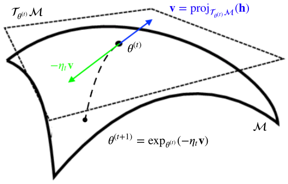
Another equivalent way of seeing the gradient update is the following: The mapping which moves the point $\vtheta^{(t)}\in\cM$ in the initial direction $-\vv$ along a geodesic of length $\norm{\eta_t\vv}_{\vtheta^{(t)}}$ is exactly the exponential map $\exp_{\vtheta^{(t)}}(\argdot)$.

Sometimes, as mentioned by Bonnabel in [2], for computational efficiency reasons or when it’s hard to solve the differential equations to obtain the exponential map, the gradient step is also approximated through the retraction $\cR_{\vx}(\vv)$:

where the function $\proj_\cM$ is the orthogonal projection from the ambient space (that includes the tangent space) onto the manifold $\cM$. Hence, the retraction represents a first-order approximation of the exponential map. The possible differences between parameter updates through the exponential map and the retraction are illustrated in the figure below:

Exponential Map VS Retraction

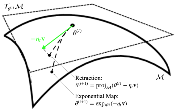
As one can see the retraction first follows a straight line in the tangent space and then orthogonally projects the point in the tangent space onto the manifold. The exponential map instead performs exact updates along to the manifold’s curved geodesics with a geodesic length that corresponds to the tangent space norm of the tangent vector $-\eta_t\vv$. Therefore, the different update methods may lead to different parameter updates. Which one is better to use depends on the specific manifold, the computational cost of the exponential map, the size of the gradient-steps and the behaviour of the loss function.

To summarize, all we need to perform RSGD is 1) the inverse of the metric tensor, 2) the formula for the orthogonal projection onto tangent spaces, and 3) the exponential map or the retraction to map tangent vectors to corresponding points on the manifold. The formulas for the steps 1)-3) vary from manifold to manifold and can usually be found in papers or other online resources. Here are few resources, that give the concrete formulas for some useful manifolds:

• Poincaré Ball: Nickel, Maximillian, and Douwe Kiela. “Poincaré embeddings for learning hierarchical representations.” Advances in neural information processing systems. 2017.

• Sphere & Hyperboloid: Wilson, Richard C., et al. “Spherical and hyperbolic embeddings of data.” IEEE transactions on pattern analysis and machine intelligence 36.11 (2014): 2255-2269.

• Birkhoff Polytope: Birdal, Tolga, and Umut Simsekli. “Probabilistic Permutation Synchronization using the Riemannian Structure of the Birkhoff Polytope.” Proceedings of the IEEE Conference on Computer Vision and Pattern Recognition. 2019.

• Grassmannian Manifold: Zhang, Jiayao, et al. “Grassmannian learning: Embedding geometry awareness in shallow and deep learning.” arXiv preprint arXiv:1808.02229 (2018).

• Several other Matrix Manifolds: Absil, P-A., Robert Mahony, and Rodolphe Sepulchre. Optimization algorithms on matrix manifolds. Princeton University Press, 2009.

Riemannian SGD on Products of Riemannian Manifolds

Since Cartesian products of Riemannian manifolds are again Riemannian manifolds, RSGD can also be applied in these product spaces. In this case, let $(\cP,\vg)$ be a product of $n$ Riemannian manifolds $(\cM_i,\vg_i)_{i=1}^n$, and let $\vg$ be the induced product metric:

Furthermore, let the optimization problem on $\cP$ be

Then, the nice thing with product spaces is that the exponential map in the product space $\cP$ simply decomposes into the concatenation of the exponential maps of the individual factors $\cM_i$. Similarly, the orthogonal projection and the gradient computations also decompose into the corresponding individual operations on the product’s factors. Hence, RSGD on products of Riemannian manifolds is simply achieved by performing the aforementioned gradient-step procedure separately for each of the manifold’s factors. A concrete algorithm for product spaces is given in the algorithm below:

Riemannian Adaptive Optimization Methods

The successful applications of Riemannian manifolds in machine learning impelled Gary Bécigneul and Octavian Ganea to further generalize adaptive optimization algorithms such as ADAM, ADAGRAD and AMSGRAD to products of Riemannian manifolds. For the details of the adaptive optimization methods I refer you to their paper [3]. A ready-to-use pytorch implementation of their proposed optimization algorithms, along with the implementation of several manifolds, has been published on github by Maxim Kochurov in his geometric optimization library called geoopt:

• Riemannian SGD

• Riemannian ADAM

We’ll use the Riemannian ADAM (RADAM) in the code-example that follows in order to see how to perform Riemannian optimization in product spaces with geoopt.

Code Example for Riemannian Optimization in Product Spaces

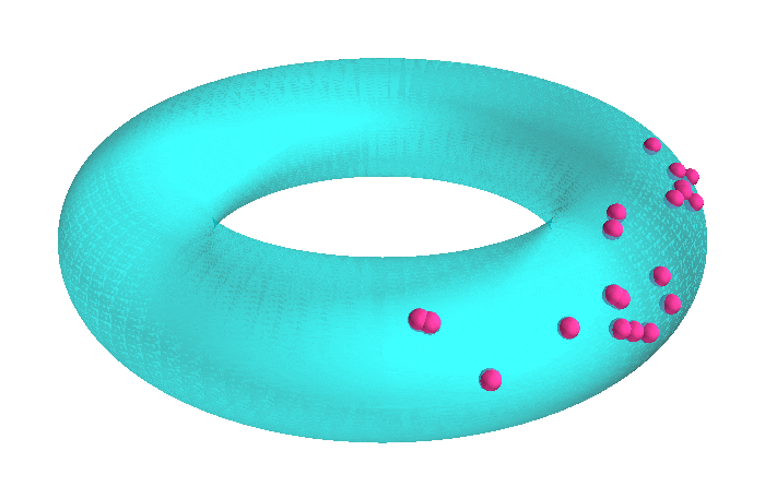
Here’s a simple code example that shows how to perform Riemannian optimization in a product space. In this example, we’ll optimize the embedding of a graph $G$ that is a cycle of $n=20$ nodes such that their original graph-distances $d_G(x_i,x_j)$ are preserved as well as possible in the geodesic distances $d_{\cP}(x_i,x_j)$ of the arrangement of the embeddings in the product space $\cP$. The product space that we’ll choose in our example is a torus (product of two circles). And the loss that we’ll optimize is just the squared loss of the graph and product space distances:

The following plot shows how the positions of the embeddings evolve over time and finally arrange in a setting that approximates the original graph distances of the cycle graph.

Evolution of Graph Embedding in Product Space

Here’s the code that shows how the optimization of this graph embedding is performed:

import torch
from geoopt import ManifoldTensor, ManifoldParameter
from geoopt.manifolds import SphereExact, Scaled, ProductManifold
from geoopt.optim import RiemannianAdam
import numpy as np
from numpy import pi, cos, sin
from mayavi import mlab
import imageio
from tqdm import tqdm

# CREATE CYCLE GRAPH ###########################################################


# Here we prepare a graph that is a cycle of n nodes. We then compute all pair-

# wise graph distances because we'll want to learn an embedding that embeds the

# vertices of the graph on the surface of a torus, such that the distances of

# the induced discrete metric space of the graph are preserved as well as

# possible through the positioning of the embeddings on the torus.


n = 20

training_examples = []
for i in range(n):
    # only consider pair-wise distances below diagonal of distance matrix
    
    for j in range(i):
        # determine distance between vertice i and j
        
        d = i-j
        if d > n//2:
            d = n-d
        # scale down distance
        
        d = d * ((2 * pi * 0.3) / (n-1))
        # add edge and weight to training examples
        
        training_examples.append((i,j,d))

# the training_examples now consist of a list of triplets (v1, v2, d)

# where v1, v2 are vertices, and d is their (scaled) graph distance


# CREATION OF PRODUCT SPACE (TORUS) ############################################


# create first sphere manifold of radius 1 (default)

# (the Exact version uses the exponential map instead of the retraction)

r1 = 1.0
sphere1 = SphereExact()

# create second sphere manifold of radius 0.3

r2 = 0.3
sphere2 = Scaled(SphereExact(), scale=r2)

# create torus manifold through product of two 1-dimensional spheres (actually

# circles) which are each embedded in a 2D ambient space

torus = ProductManifold((sphere1, 2), (sphere2, 2))

# INITIALIZATION OF EMBEDDINGS #################################################


# init embeddings. sidenote: this initialization was mostly chosen for

# illustration purposes. you may want to consider better initialization

# strategies for the product space that you'll consider.

X = torch.randn(n, 4).abs()*0.5

# augment embeddings tensor to a manifold tensor with a reference to the product

# manifold that they belong to such that the optimizer can determine how to

# convert the the derivatives of pytorch to the correct Riemannian gradients

X = ManifoldTensor(X, manifold=torus)

# project the embeddings onto the spheres' surfaces (in-place) according to the

# orthogonal projection from ambient space onto the sphere's surface for each

# spherical factor

X.proj_()

# declare the embeddings as trainable manifold parameters

X = ManifoldParameter(X)

# PLOTTING FUNCTIONALITY #######################################################


# array storing screenshots

screenshots = []

# torus surface

phi, theta = np.mgrid[0.0:2.0 * pi:100j, 0.0:2.0 * pi:100j]
torus_x = cos(phi) * (r1 + r2 * cos(theta))
torus_y = sin(phi) * (r1 + r2 * cos(theta))
torus_z = r2 * sin(theta)

# embedding point surface

ball_size = 0.035
u = np.linspace(0, 2 * pi, 100)
v = np.linspace(0, pi, 100)
ball_x = ball_size * np.outer(cos(u), sin(v))
ball_y = ball_size * np.outer(sin(u), sin(v))
ball_z = ball_size * np.outer(np.ones(np.size(u)), cos(v))


def plot_point(x, y, z):
    point_color = (255/255, 62/255, 160/255)
    mlab.mesh(x + ball_x, y + ball_y, z + ball_z, color=point_color)


def update_plot(X):

    # transform embedding (2D X 2D)-coordinates to 3D coordinates on torus
    
    cos_phi = X[:,0] * r1
    sin_phi = X[:,1] * r1
    xx = X[:,0] + cos_phi * X[:,2] * r2
    yy = X[:,1] + sin_phi * X[:,2] * r2
    zz = r2 * X[:,3]

    # create figure
    
    mlab.figure(size=(700, 500), bgcolor=(1, 1, 1))

    # plot torus surface
    
    torus_color = (0/255, 255/255, 255/255)
    mlab.mesh(torus_x, torus_y, torus_z, color=torus_color, opacity=0.5)

    # plot embedding points on torus surface
    
    for i in range(n):
        plot_point(xx[i], yy[i], zz[i])

    # save screenshot
    
    mlab.view(azimuth=0, elevation=60, distance=4, focalpoint=(0, 0, -0.2))
    mlab.gcf().scene._lift()
    screenshots.append(mlab.screenshot(antialiased=True))
    mlab.close()

# TRAINING OF EMBEDDINGS IN PRODUCT SPACE ######################################


# build RADAM optimizer and specify the embeddings as parameters.

# note that the RADAM can also optimize parameters which are not attached to a

# manifold. then it just behaves like the usual ADAM for the Euclidean vector

# space. we stabilize the embedding every 1 steps, which rthogonally projects

# the embedding points onto the manifold's surface after the gradient-updates to

# ensure that they lie precisely on the surface of the manifold. this is needed

# because the parameters may get slightly off the manifold's surface for

# numerical reasons. Not stabilizing may introduce small errors that accumulate

# over time.

riemannian_adam = RiemannianAdam(params=[X], lr=1e-2, stabilize=1)

# we'll just use this as a random examples sampler to get some stochasticity

# in our gradient descent

num_training_examples = len(training_examples)
training_example_indices = np.array(range(num_training_examples))
def get_subset_of_examples():
    return list(np.random.choice(training_example_indices,
                                 size=int(num_training_examples/4),
                                 replace=True))

# training loop to optimize the positions of embeddings such that the

# distances between them become as close as possible to the true graph distances

for t in tqdm(range(1000)):

    # zero-out the gradients
    
    riemannian_adam.zero_grad()

    # compute loss for next batch
    
    loss = torch.tensor(0.0)
    indices_batch = get_subset_of_examples()
    for i in indices_batch:
        v_i, v_j, target_distance = training_examples[i]
        # compute the current distances between the embeddings in the product
        
        # space (torus)
        
        current_distance = torus.dist(X[v_i,:], X[v_j,:])
        # add squared loss of current and target distance to the loss
        
        loss += (current_distance - target_distance).pow(2)

    # compute derivative of loss w.r.t. parameters
    
    loss.backward()

    # let RADAM compute the gradients and do the gradient step
    
    riemannian_adam.step()

    # plot current embeddings
    
    with torch.no_grad():
        update_plot(X.detach().numpy())

# CREATE ANIMATED GIF ##########################################################


imageio.mimsave(f'training.gif', screenshots, duration=1/24)

Of course, one might choose better geometries to embed a cycle graph. Also, a better embedding could have been achieved if the embeddings had wrapped around the curved tube of the torus. This example was mostly chosen to have an illustrative minimal working example in order to get you started Riemannian optimization in product spaces. A paper that extensively studies the suitability of products of spaces of constant curvature to learn distance-preserving embeddings of real-world graphs is the work of Gu et al. [4].

That’s all for now, I hope that my motivation and explanation of RSGD was helpful to you and that you are now ready to get started with Riemannian optimization.

References

1. A. Douik and B. Hassibi, “Manifold Optimization Over the Set of Doubly Stochastic Matrices: A Second-Order Geometry,” arXiv preprint arXiv:1802.02628, 2018.
2. S. Bonnabel, “Stochastic gradient descent on Riemannian manifolds,” IEEE Transactions on Automatic Control, vol. 58, no. 9, pp. 2217–2229, 2013.
3. G. Bécigneul and O.-E. Ganea, “Riemannian adaptive optimization methods,” arXiv preprint arXiv:1810.00760, 2018.
4. A. Gu, F. Sala, B. Gunel, and C. Ré, “Learning Mixed-Curvature Representations in Product Spaces,” 2018.