An Overview of Collaborative Filtering Algorithms for Implicit Feedback Data

This blogpost gives an overview of today’s most predominant types of recommender systems for collaborative filtering from implicit feedback data. The overview is by no means exhaustive, but it should provide the reader with a good overview about the topic.

First, some background about recommender systems is given. Also, the setting of collaborative filtering from implicit feedback data is defined and the typical application structure of a recommender service is explained. Then, several collaborative filtering models are described in more detail together with a discussion on their advantages and disadvantages. Finally, a summary of the different approaches is given. A slide deck accompanying the article can be found here:

Background on Recommender Systems

Recommender systems are at the heart of any of today’s large-scale e-commerce, news, content-streaming, dating or search platforms. A critical success factor of such platforms is the ability to reduce the overwhelming amount of options to a few relevant recommendations matching the users’ individual and trending interests.

According to McKinsey & Company, 35% of the consumer purchases on Amazon and 75% of the views on Netflix in 2012 came from product recommendations based on recommendation engines [1]. Goodwater Capital [2] also reports that in 2017, 31% of the tracks listened on Spotify stemmed from personalized playlists generated by Spotify’s recommender system. These numbers clearly demonstrate the significance of algorithmic recommendations in online services.

Connecting customers to products that they love is critical to both, the customers and the companies. Because if users fail to find the products that interest and engage them, they tend to abandon the platforms [3]. In a report about the business-value of their recommender algorithms Netflix describes how the reduction of the monthly churn both increases the lifetime value of existing subscribers, and reduces the number of new subscribers that they need to acquire to replace cancelled members. They estimate the combined effect of personalization and recommendations to save them more than the exorbitant amount of $1B per year [4].

The urgency of the capability to provide relevant and personalized recommendations can also be seen in the prize money of $1M that Netflix advertised in its famous “Netflix Prize” competition of 2006 for the first team that could improve the Netflix algorithm’s RMSE by 10% [5]. The competition inspired a multitude of researchers to participate and to contribute to the development of next-generation recommender systems. In the end, the grand prize was won by Yehuda Koren, Robert Bell and Chris Volinsky in 2009 who had developed a model that blended the predictions of hundreds of predictors, including a plethora of matrix factorization models, neighbourhood models and restricted Boltzmann machines [6].

Ironically, in 2012 Netflix published in a blogpost of theirs [7] that they never happened to use Koren et al.’s algorithm in production due to its engineering costs: “the additional accuracy gains that we measured did not seem to justify the engineering effort needed to bring them into a production environment.” Anyways, the field of recommender systems has certainly profited from the inventions that were sparked by virtue of the competition.

The Collaborative Filtering Setting

Many different types of recommender systems have evolved over the years. One way to characterize recommender systems is through the information that they consider to produce their rankings:

• Collaborative Filtering: In collaborative filtering the recommender system purely learns form the interaction patterns between users and items [8]. The contents and features of the items and users are completely ignored. Users and items are just treated as enumerated nodes of an undirected (weighted or unweighted) bipartite graph $G=(U\cup I, E)$ where the items $I$ are indexed as $i_1,…,i_{\card{I}}$ and the users $U$ are indexed as $u_1,…,u_{\card{U}}$. Nothing more than the vertices, edges $\set{u_j,i_k}$ and maybe a some edge weights $w_{u_j,i_k}$ are known. Hence collaborative filtering corresponds to predicting promising links from user nodes to item nodes based on the observed common connection patterns. It is called collaborative filtering, because in the collaborative filtering approaches it is commonly assumed that learning the interaction patterns of one user (e.g., the items a user has interacted with) will help to predict relevant items for another user that has a similar interaction pattern (in terms of interacted items) as the latter user. Hence it is as if users were collaborating to produce the rankings of items for each other.

• Content-Based: In content-based recommender systems, the recommender system additionally learns from the content and features of the items (e.g., image location and data or text data) and sometimes also from the features of the users, to produce a list of rankings as done for example in [9].

• Context-Aware: These recommender systems include additional information about a user’s context [10], e.g., whether the user is accessing the service from a mobile or desktop client, his current geolocation, his current time of day, whether the user is stationary or travelling, or whether the user is in a quiet or noisy place.

This blogpost is purely concerned with the collaborative filtering setting. However, most of the collaborative filtering approaches can usually be extended to include the other aforementioned information sources, as for example done in the approach of [9].

Explicit VS Implicit Feedback Data

The training of recommender systems relies on data that is gathered from the feedback that users gave to items. This feedback can be divided into two categories as defined in [11]:

• Explicit Feedback: Here a user explicitly gives a rating to an item on a certain scale.

• Implicit Feedback: Here a user implicitly provides the information about the relevance of an item by interacting with it according to a certain notion of time, e.g., a certain amount of times, or a total amount of time, or the percentage watched of a movie.

The relevance of algorithms capable of dealing with implicit feedback data can be motivated by the natural abundance of implicit feedback data versus the usual scarcity of explicit feedback data [12]. This blogpost is purely concerned with binary implicit feedback data, as done in most of the academic literature.

Recommender Service: An Interplay of a Retrieval and a Ranking System

Before looking at our first concrete collaborative filtering model, let’s first have a look at how a recommender service is usually structured. A common practice [13] is to structure a recommendation service into two components as follows :

1. A retrieval system that retrieves potential relevant items in a very efficient manner (e.g., KD-trees [14]), maximum inner product search (MIPS) [15], locality-sensitive hashing (LSH) [16, 17, 18], or also neural-network based methods [12].

2. A ranking system, which we also refer to as recommender system, which usually runs a more expensive and sophisticated algorithm to precisely rank the retrieved potential positive candidates such that they can be presented in their final estimated relevance order to a user [12].

The figure below illustrates the interplay of a retrieval and a ranking system. Whether to use just a recommender system, or a combination of a retrieval and recommender system depends on the size of the data (in terms of number of users and items) and the computational cost of the recommender system. If the ranking has a high computational cost, and there are lots of items, then it makes sense to have a retrieval system that retrieves a subset of potential candidates in a cheap way. An important thing to note here is that, besides the ranking accuracy of the ranking system, also the quality of the subsample retrieved by the retrieval system strongly affects the performance metrics of the entire recommender service.

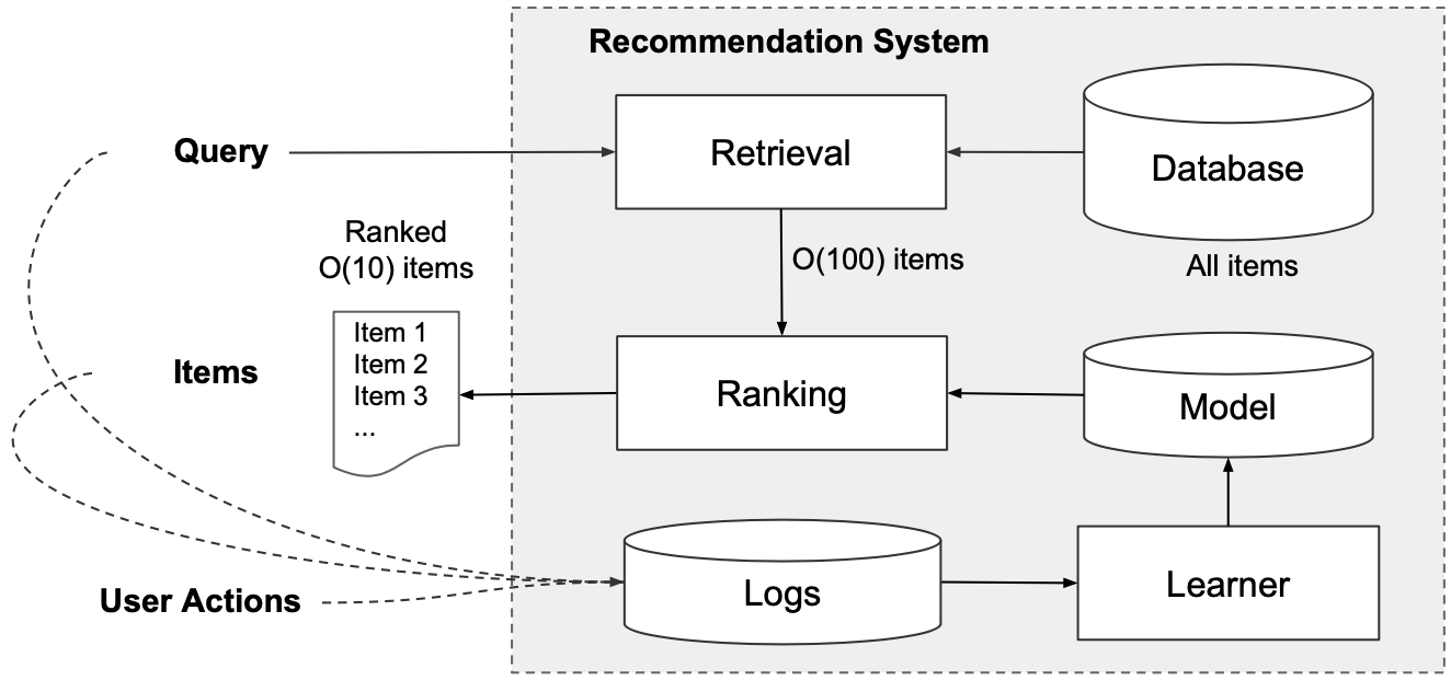
In the collaborative filtering setting, the query is just a user index and the result is a ranked list of indices of recommended items. As depicted, the retrieval system usually returns a subset in the order of $N=100$ items to the ranking system.

Now that we have enough background on recommender systems we can have a look at the first collaborative filtering model.

Item Popularity

The Item Popularity model is a very simple and efficient ranking model that simply recommends items based on their popularities. The more popular an item is, the higher up it is on its recommendation list. Thus, the ranking of an item $i$ for user $u$ is simply computed through

$$\hat{x}_{ui}=\frac{\#\text{interactions with item }i}{\# \text{interactions in total}}.$$

Hence, it completely ignores the user’s features, which can be disadvantageous if one wants to create recommendations tailored to a user’s preferences.

Nevertheless, it can be a very powerful prediction model. Its strengths lie in its simplicity and its efficiency. The Item Popularity model can be particularly useful in situations where there is little information known about a user’s preferences. Therefore, it is often used to overcome the cold-start problem.

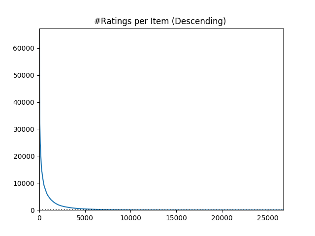
A reason why the Item Popularity model works quite well in practice is because, usually, the popularity of items is distributed according to a power-law: most of the interactions happen with a few popular items, and the rest of the items only have a few interactions. The following plot illustrates how the number of interactions per item is distributed according to a power-law for the Movielens-20M dataset.

Matrix Factorization (MF)

Matrix factorization (MF) predicts the relevance $\hat{x}_{ui}$ of an item $i\in I$ for a user $u\in U$ through the dot product

$$\hat{x}_{ui}=\scprod{\vx_u,\vx_i},$$

where $\vx_u$ and $\vx_i$ are $d$-dimensional representations of the user $u$ and item $i$ in a latent factor space. These latent factor representations of users and items are the parameters $\vtheta$ that are aimed to be learned:

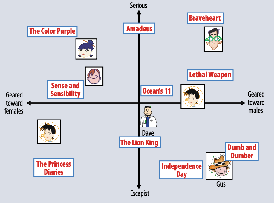
Several works showed how these latent factor space dimensions tend to capture concepts of users and items, e.g., “male” or “female” for users, or “serious” vs “escapist” for movies as illustrated below from the work of [5].

For explicit feedback data the parameters are trained by minimizing the squared loss over the observed rankings $x_{ui}$ of the interaction matrix $\MX\in\R^{\card{U}\times\card{I}}$, collected as training instances $(u,i)\in\cD$:

Some approaches for implicit feedback data, such as [19, 20], rely on binarization and imputation of the unobserved entries of $\MX$ as 0, turning the optimization problem into

$$\cL(\vtheta)=\norm{\MX - \MX_U\MX_I^T}_2^2.$$

The latter loss clearly shows why the recommender system approach has its name matrix factorization. Under some conditions, one can assume that $\rank(\MX_U\MX_I^\T)\leq d$, making the problem tightly related to Singular Value Decomposition (SVD) and Principal Component Analysis (PCA).

Other approaches for implicit feedback data argue that one should still impute the non-observed interactions as $0$, but weigh the prediction errors for observed and unobserved interactions differently. Such approaches fall under the category of weighted regularized matrix factorization (WMRF), having a training loss of the form

$$\cL(\vtheta) = \sum_{(u,i)\in\cD} c_{ui}(x_{ui}-\hat{x}_{ui})^2.$$

where the weights $c_{ui}$ are chosen according to a weighting-strategy. Hu et al. [8], Pan et al. [21] and He et al. [22], proposed various weighting-schemes that all assign a fixed weight $c_{ui}=1$ to the observed interactions, and the weights $c_{ui}$ for the unobserved interactions are chosen according to one of the following strategies:

• Uniform-Weighting: Chooses some fixed weight $c_{ui}\in[0,1)$, meaning that all unobserved interactions share the same probability of being negative examples.
• User-Activity Based: Chooses the weight based on the number of ratings that a user $u$ gave: $c_{ui}\propto\norm{\vx_u}_1$. With the argument that, the more a user has interacted with the system, the more confident one can be about the inferred irrelevance of the user’s left-out items.
• Item-Popularity Based: Assigns lower weights to popular items. The rationale behind this is: the more popular an item is, the more likely it is to be known. Hence, a non-interaction on a popular item is more likely to be due to its true irrelevance to a user.

Other more advanced models also train a global bias $\mu$, and user- and item-specific biases $\mu_u$ and $\mu_i$ to predict the rankings as

$$\hat{x}_{ui}=\scprod{\vx_u,\vx_i}+\mu_u+\mu_i+\mu.$$

This aims to compensate for the systematic tendencies that some users tend to give higher ratings than others, and some items tend to receive higher ratings than others. The rationale behind this is that the latent concepts (the $d$-dimensions of the latent factor space) should not be used to explain these systematic tendencies [5].

It is also a common practice to regularize the user- and item-embeddings and the means with L2-regularization

This form of regularization can also be motivated from a probabilistic perspective where the user- and item-embeddings and the means are assumed to be distributed according to multivariate Gaussian distributions in the latent factor space. For a derivation see [23].

In the famous Netflix Prize, launched in 2006, the majority of the successful recommender systems were using matrix-factorization approaches [3]. For many years, matrix factorization has been the ranking model of first-choice and a lot of improvements and extensions have been proposed, including:

• Alternating Least-Squares (ALS): Various alternating least-squares (ALS) optimization approaches, such as eALS [22] and ALS-WR [24], have been developed. These approaches aim to speed-up the convergence of the non-convex optimization problem through the surrogate of two convex optimization problems. ALS works through the following alternation: at each iteration, once the user embeddings are fixed and the solutions for the items are obtained in a closed-form, and vice-versa.

• Including Temporal Dimensions: Another direction of work, e.g. [25, 26], has been concerned with incorporating temporal dimensions into matrix factorization. These approaches model the trends of items and the changes of users’ tastes by expressing the user and item embeddings, and also the biases, as functions of time.

• Non-Negative Matrix Factorization: For some ranking applications it might be desirable to only have predictions that are positive. To this end, several works have been concerned with applying non-negative matrix factorization to collaborative filtering, including [27, 28].

• On-line Learning and Regret Bounds: A lot of effort has also been invested in the development of on-line learning algorithms (e.g. [22, 29]) and the derivation of regret bounds (e.g. [30, 31]), making it possible to scale matrix factorization to big-data settings with on-line learning and convenient regret bounds.

Note that while all examples here have been using the squared loss, matrix factorization can also be trained using the pair-wise BPR loss as done in [32].

All-in-all, matrix factorization has demonstrated to be a powerful and successful recommender model. Indeed, it had been successfully used to do YouTube video recommendations, until it got replaced by neural network approaches recently [12]. The fact that, at its heart, matrix factorization only uses a bi-linear form to predict the rankings, makes it computationally very attractive. However, as we will see in what follows, recent state-of-the-art approaches critique the inner product for failing at propagating similarities [9] and for being too rigid, in the sense that it is only a bi-linear form as opposed to a more powerfulnon-linear prediction function [33].

Collaborative Metric Learning (CML)

Metric learning approaches aim to learn a distance metric that assigns smaller distances between similar pairs, and larger distances between dissimilar pairs. Collaborative Metric Learning (CML) [9] advocates the embedding of users and items for recommender systems in metric spaces in order to exploit a phenomenon called similarity propagation. In their work, Hsieh et al. [9] explain how similarity propagation is achieved due to the fact that a distance metric $d$ must respect, amongst several other conditions, the crucial triangle-inequality:

$$\forall x,y,z\colon \quad d(y,z)\leq d(x,y) + d(x,z).$$

This implies that, given the information that “$x$ is similar to both $y$ and $z$” the learned metric $d$ will not only pull the pairs $y$ and $z$ close to $x$, but also pull $y$ and $z$ relatively close to one-another. Thus, the similarity of $(x,y)$ and $(x,z)$ is propagated to $(y,z)$.

The authors critique that, since matrix factorization is using the inner-product, and the inner-product does not necessarily respect the triangle inequality (e.g., violation for $x=-1$, $y=z=1$), such a similarity propagation is not happening in matrix factorization approaches. An illustration of how the inner-product fails at propagating similarities even for a simple interaction matrix is given below:

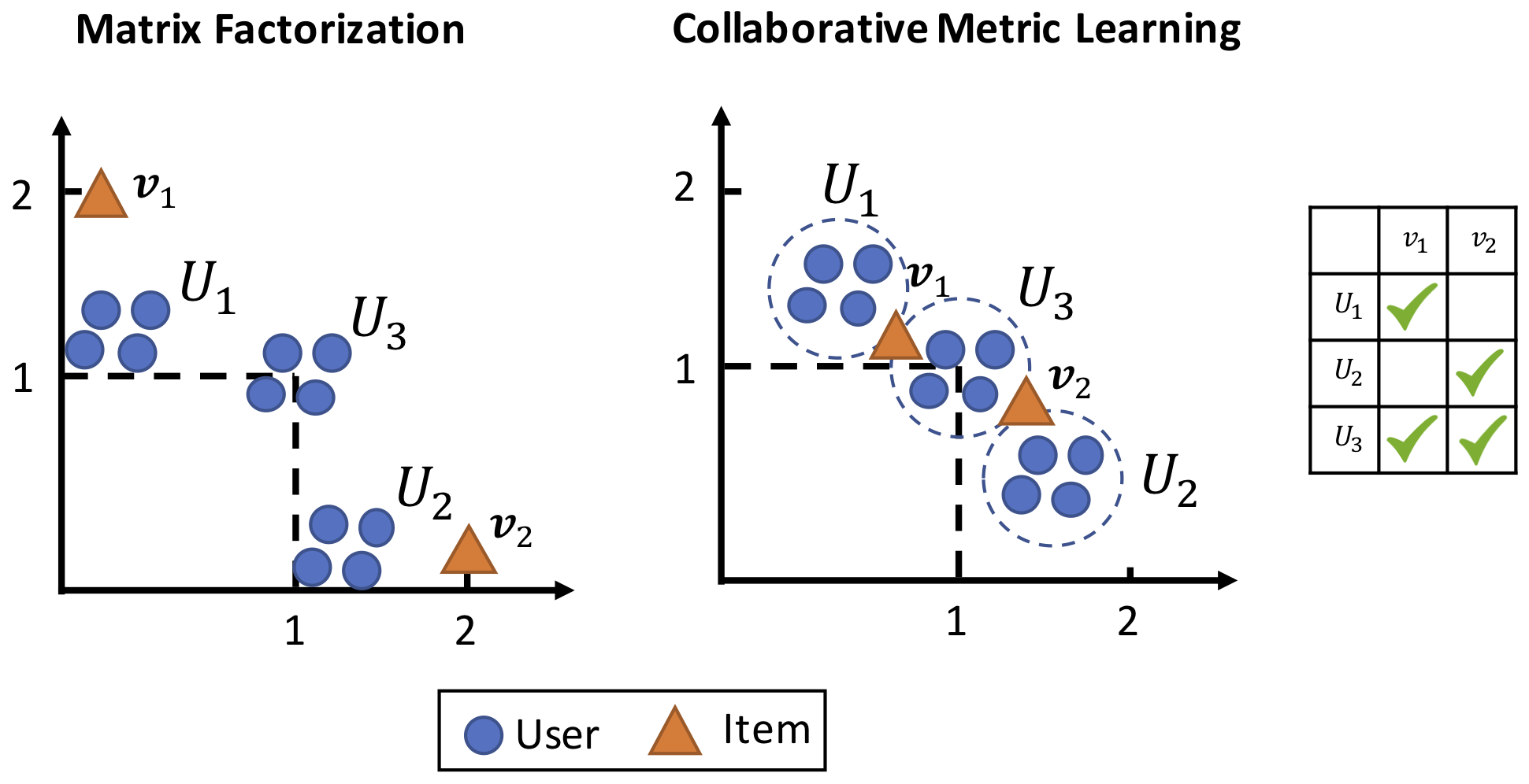
The great convenience of encoding users and items in a metric space $(\cM,d)$ is that the joint metric space does not only encode the similarity between users and items, but it can also be used to determine user-user and item-item similarities. This improves the interpretability of the model, as opposed to a model that relies on the inner product to compute similarities. What matrix factorization approaches usually do to compensate for this lack is to compute user-user or item-item similarities using the cosine-distance. However as illustrated in the figure above, this doesn’t yield optimal results.

Hopefully, by now the reader should be convinced that similarity propagation is a desirable property to have in order to generalize from the observed user-item interactions to unseen pairs of interactions and user-user and item-item similarities. Next, we’ll look at how the training of the embeddings is performed in CML.

The embedding training approach of of CML is to pull positive user-item pairs close together and to push negative user-item pairs far apart according to some margin. This process will then cluster users who co-like the same items together, and also cluster the items that are co-liked by the same users together. Eventually, a situation is reached where the nearest neighbours of any user $u$ will become:

• the items the user $u$ liked, and
• the items liked by other users who share a similar taste with user $u$.

Therefore, learning from the observed positive interactions propagates these relationships also to user-user and item-item pairs for which there are no observed relationships.

In CML the relevances then are simply predicted as the negative distance

$$\hat{x}_{ui}=-d(\vx_u,\vx_i),$$

meaning that a closeby item as a higher ranking than an item that is farther away. The optimization objective trained to achieve the aforementioned desiderata is the following:

$$\cL(\vtheta) = \cL_m(\vtheta) + \lambda\Omega(\vtheta) \quad \text{s.t. } \norm{\vx_*}\leq 1,$$

where the various loss terms have the following meanings:

• The term $\cL_m(\vtheta)$ is the WARP loss of the predicted rankings, given by the negative metric space distances $\hat{x}_{ui}=-d(\vx_u,\vx_i)$ and $\hat{x}_{uj}=-d(\vx_u,\vx_j)$:

  $$ \cL_m(\vtheta)=\sum_{(i,j)\in\cS}\sum_{(u,k)\nin\cS} w_{ij}\left[m+d(\vx_u,\vx_i)^2-d(\vx_u,\vx_j)^2\right]_+. $$
  $$ \cL_m(\vtheta)=\sum_{(i,j)\in\cS}\sum_{(u,k)\nin\cS} w_{ij}\left[m+d(\vx_u,\vx_i)^2-d(\vx_u,\vx_j)^2\right]_+. $$

  The set $\cS$ is the set of observed positive interactions. The gradients caused by the WARP loss for a user $u$ and its positive and negative items are illustrated in the figure below.

  

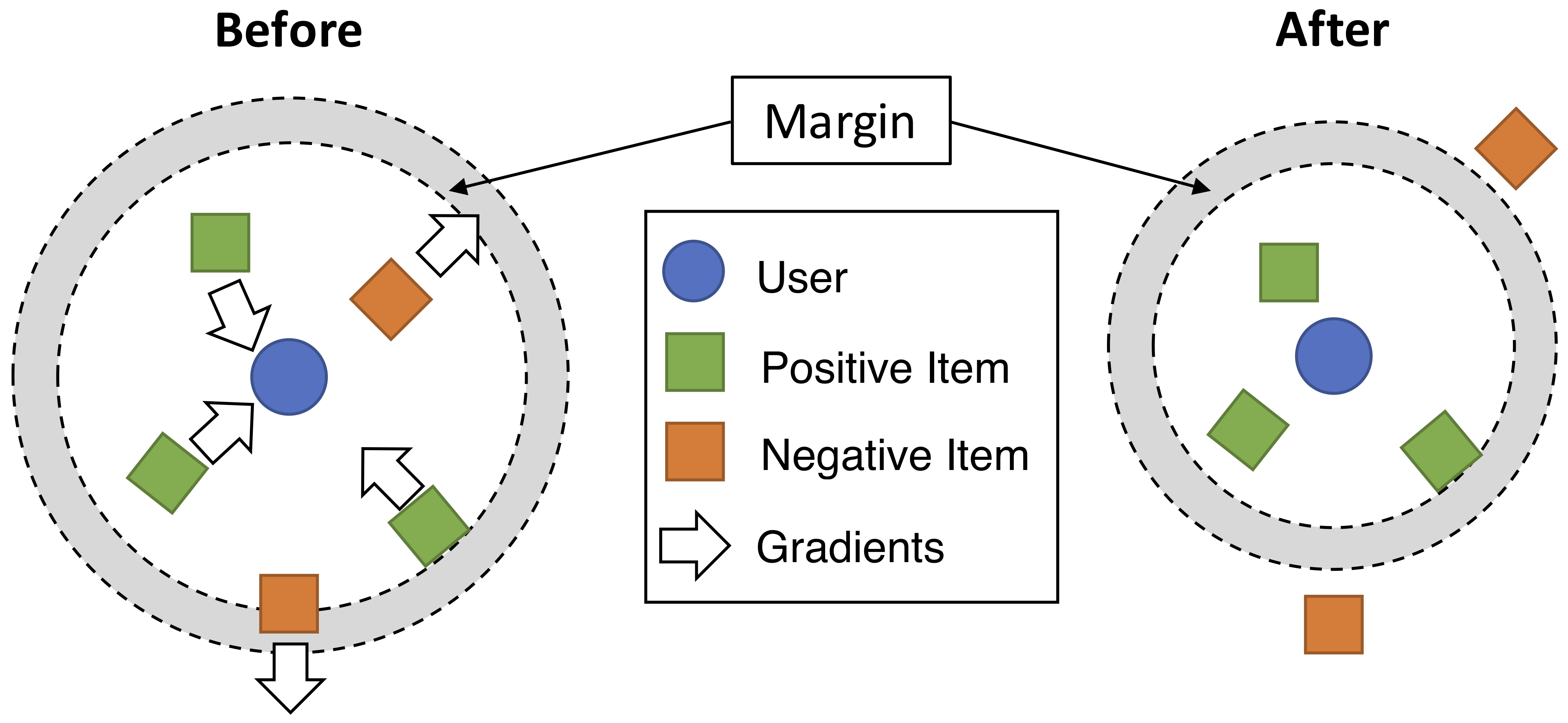  The figure by [9] shows the gradients created by the WARP loss in CML. For the positive items of a user, gradients are created to pull them closer until they lie within a certain margin $m$ to the user. For the negative items of a user, gradients are created to push them away until they lie far away from the user, outside a ball of radius $m$, where $m$ is the margin, usually chosen as $1$.

• The regularization term $\Omega(\vtheta)$ uses covariance regularization as proposed by Cogswell et al. [34].

  $$\Omega(\vtheta)=\norm{\MSigma - \diag(\MSigma)}_2^2,$$

  where $\MSigma$ is the covariance matrix of the concatenation of all the user and item embeddings. This de-correlates the dimensions of the metric space. Since covariances can be seen as a measure of linear redundancy between dimensions, this loss essentially tries to prevent each dimension from being redundant by penalizing off-diagonal entries in the covariance matrix and thus encouraging the embeddings to efficiently utilize the given space. The covariance matrix is computed as follows: Let $\MY$ be the concatenation of the $d$-dimensional user and item-embeddings $\MX_U$ and $\MX_I$:

  $$\MY=\begin{bmatrix} \MX_U\\ \MX_I \end{bmatrix} \in\R^{(\card{U}+\card{I})\times d}.$$

  The mean embedding vector is then computed as

  $$ \vmu := \frac{1}{\card{U}+\card{I}}\sum_{i=1}^{\card{U}+\card{I}} \MY_{i,:}\in\R^{1\times d}, $$
  $$ \vmu := \tfrac{1}{\card{U}+\card{I}}\sum_{i=1}^{\card{U}+\card{I}} \MY_{i,:}, $$

  and the covariance matrix $\MSigma$ is obtained via

  $$ \MSigma = \frac{1}{\card{U}+\card{I}} \sum_{i=1}^{\card{U}+\card{I}} \left(\MY_{i,:}-\vmu\right)^\T \left(\MY_{i,:}-\vmu\right)\in\R^{d\times d}. $$
  $$ \MSigma = \tfrac{1}{\card{U}+\card{I}} \sum_{i=1}^{\card{U}+\card{I}} \left(\MY_{i,:}-\vmu\right)^\T \left(\MY_{i,:}-\vmu\right). $$

• The optimization constraint $\norm{\vx_{*}}\leq 1$ forces all user and item embeddings $\vx_{*}$ to stay within a unit-sphere in order to easily apply locality sensitive hashing (LSH) [16] later. L2-regularization is intentionally avoided, as this would just pull the embeddings towards the origin. The authors argue that in the metric space the origin does not have any specific meaning.

One great advantage of CML is that it can the recommendations can be easily performed on massive datasets. Since CML uses the Euclidean distance to represent the relevances, it can be used with off-the-shelf LSH. In contrast, matrix factorization approaches would have to use approximate Maximum Inner Product Search (MIPS), which is considered to be a much harder problem than LSH [15]. A disadvantage of CML might be that the distance function itself might not be expressive enough to represent the complex user-item relevance relationships, which might be modeled through arbitrary non-linear interaction functions as suggested in some approaches that follow later.

Still, the example of CML clearly illustrated the benefits obtained through similarity propagation when learning a distance metric to predict the relevances. This also motivates the next recommender system approaches, which also learn distance metrics in hyperbolic space to predict rankings.

Hyperbolic Recommender Systems

So far, three approaches [35, 36, 37] harnessing hyperbolic geometry for recommender systems have been published. Both approaches represent users and items in hyperbolic geometry and predict the relevance between users and items as

$$\hat{x}_{ui}=\alpha d(\vx_u,\vx_i),\quad\text{with }\alpha<0,$$

where $\vx_u$ and $\vx_i$ are the trained user and item-embeddings, lying in hyperbolic geometry, and $d$ is the geodesic distance function in hyperbolic geometry.

Since all approaches use distance metrics to represent the relevance relationships between users and items they all fall under the category of metric learning approaches, just as the aforementioned CML. Therefore, they also benefit from the similarity propagation phenomenon, as the hyperbolic geodesic distance also has to respect the triangle inequality.

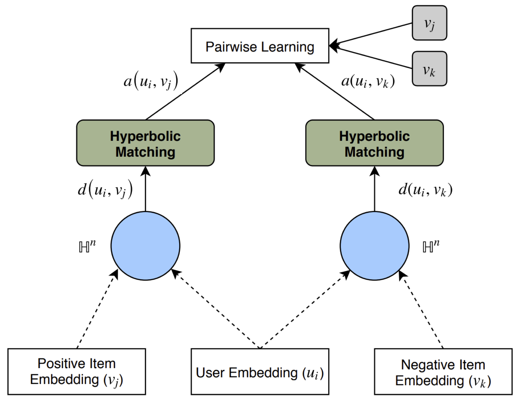
The approaches of [35, 36, 37] train their embeddings via the BPR loss [32], yielding the optimization objective

where the parameters $\vtheta$ consist of the user embeddings $\MX_U$, the item embeddings $\MX_I$ and the scalar $\alpha$. In some of their experiments [36] also use the WMBR [38] loss. The embeddings are trained via the Riemannian optimization used with hyperbolic spaces. An illustration of the architecture of the pairwise learning approach is given in the figure below.

Even though Vinh et al. [35] use the Poincaré ball, and Chamberlain et al. [36] use the hyperboloid as their model for hyperbolic geometry, the two approaches can be considered as practically equivalent. The only real difference is that Chamberlain et al. further apply some L2-regularization on the user and item embeddings.

Chamberlain et al. [36] further explored the possibilities of expressing users as the Einstein midpoint $\vmu$ (corresponding to a mean) of their positively interacted items in order to reduce the amount of learned parameters.

In their experiments, Chamberlain et al. showed that expressing the users as the midpoint of their interacted items can speed-up the training, due to the reduced amount of parameters, without sacrificing the model’s recommendation performance. Such an approach is particularly useful for asymmetric datasets that contain much more users than items ($\card{U}\gg\card{I}$).

The third hyperbolic recommender system approach of Schmeier et al. [37] embedded their entities using a different loss

$$\cL(\vtheta) = - \sum_{(u,i)\in\cD} \log\left( \frac{ e^{\hat{x}_{ui}} }{ e^{\hat{x}_{ui}} + \sum_{(u,j)\in\cD'} e^{\hat{x}_{uj}} } \right),$$

where $\cD$ is the dataset of positive interactions and $\cD’$ is a set of $K$ negative interactions for user $u$, obtained through negative sampling. This loss also encourages that relevant user-item paris are closeby, and irrelevant user-item pairs are farther apart. Also, this is exactly the same loss that was used by Nickel & Kiela [39] to train a graph-embedding for the representation of hypernymy relations in hyperbolic space.

To conclude, let’s discuss the advantages and disadvantages of these hyperbolic recommender models. The advantages of these metric learning approaches are the same as the ones of CML: the most important one being that they all profit from similarity propagation and thus simultaneously learn user-user and item-item similarity. Furthermore, as revealed in the experiments of three approaches, the choice of a hyperbolic geometry turned out to provide a good bias for the representations. One can also imagine that one could perform fast nearest-neighbour search for massive datasets through a generalization of LSH to hyperbolic space. Similarly as to CML, these approaches have the disadvantage that the distance function might not be powerful enough to express the user-item relevance relationships entirely. It might be that this relationship is even better modeled through a non-linear interaction function as suggested in the next approach.

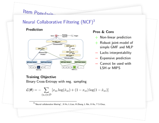
Neural Collaborative Filtering (NCF)

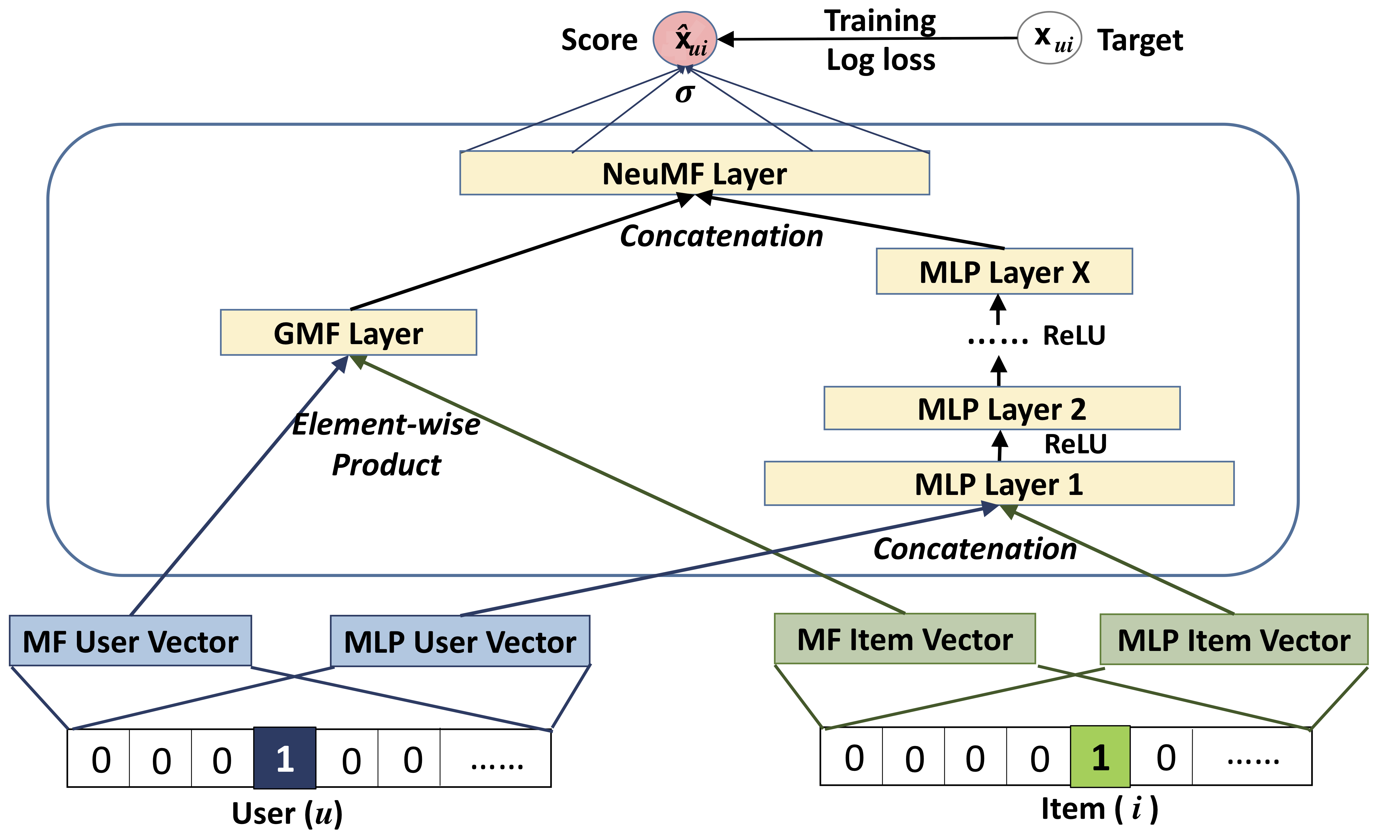
In contrast to the bi-linear prediction function used with matrix factorization, or a rigid distance function as used with the metric learning approaches, Neural Collaborative Filtering (NCF), introduced by He et al. [33], aims to learn a non-linear interaction function acting on trained user and item embeddings to predict the relevances. The non-linear interaction function is implemented through two models that are trained jointly:

• Generalized Matrix Factorization (GMF): representing a generalization of the inner-product, where the products in the inner product are further scaled by individual factors.

• Multi-Layer Perceptron (MLP): a pyramidal 3-layer perceptron with ReLU activations.

The ranking $\hat{x}_{ui}$, representing the relevance of item $i\in I$ for a user $u\in U$ is computed as follows:

• First, the user and item embeddings, that are also learned, are retrieved for each of the two joint models:

  $$\vx_u^{GMF}, \vx_i^{GMF},\qquad \vx_u^{MLP}, \vx_i^{MLP}.$$

• Then, the interaction for GMF is computed by building the element-wise product of the corresponding user and item embedding vectors. Then a weighted sum of the product’s coefficients is computed through a parameter $\vh$ and also a bias is added:

  $$\hat{x}_{ui}^{GMF}=\vh^T\left(\vx_u^{GMF}\odot \vx_i^{GMF}\right) + b^{GMF}.$$

  Note how for $\vh=(1,\ldots,1)^\T$ and $b^{GMF}=0$ the GMF model recovers the usual dot-product that is used in matrix-factorization.

• Then, the interaction for the MLP is computed by concatenating the corresponding user and item embeddings and passing them through the pyramidal 3-layer perceptron with ReLU activations. Also, a bias is added:

  $$\hat{x}_{ui}^{MLP}=\text{MLP}(\vx_{u}^{MLP}, \vx_{i}^{MLP}) + b^{MLP}.$$

• In order to weigh the importance of both models, the results of GMF and the 3-MLP may be scaled by factors $\alpha$ and $(1-\alpha)$, where $\alpha\in(0,1)$. In their proposed architecture He et al. fixed $\alpha=0.5$. Finally, the ranking $\hat{x}_{ij}$ is obtained by building a convex combination of the activations $\hat{x}_{ui}^{GMF}$ and $\hat{x}_{ui}^{MLP}$, and then and passing the result through the sigmoid function:

  $$\hat{x}_{ui}=\sigma\left( \alpha \hat{x}_{ui}^{GMF} + (1-\alpha)\hat{x}_{ui}^{MLP} \right).$$

An illustration of the architecture of NCF is given in the figure below. The models GMF and MLP can also be instantiated on their own, while the sigmoid output function is maintained.

In their experiments He et al. trained NCF using the binary cross-entropy loss with negative sampling. One could also use the pair-wise BPR loss to train the model’s parameters, however, in their experiments He et al. observed better performance metrics with the binary cross-entropy loss and negative sampling:

where the training instances $(u,i)\in\cD$ consist of positive and negative interactions. The negative interactions are oversampled according to a negative sampling factor of $K$, where $K=5$ turned out to work well for both datasets (Movielens-1M and Pinterest) for the datasets used in the experiments of He et al.

While the models GMF and MLP can be instantiated each on their own, the experiments of the He et al. [33] revealed that the joint model outperformed the individual models in every case. For the datasets Movielens-1M and Pinterest, their proposed architecture outperformed a state-of-the-art matrix-factorization baseline eALS [22] (alternating least-squares MF). Thus, one can argue that modeling the interaction as a non-linear function, instead of a bi-linear function, is advantageous for the accurate prediction of rankings.

The disadvantages of NCF are that, in contrast to the metric learning approaches, NCF lacks interpretability and NCF does not automatically learn user-user and item-item similarities via similarity propagation. Also, the rank prediction is rather computationally expensive and does not scale well to predictions over the the full set of items if one should desire to do so. Also, techniques like LSH and MIPS cannot be applied to its embeddings or latent representations to get fast nearest-neighbour search. However, for massive datasets it may still be used in conjunction with a retrieval system.

Autoencoders for Collaborative Filtering

Recently, autoencoders have gained momentum in the field of recommender systems. The important connection to be noticed here is that a 1-layer autoencoder with linear activation functions reduces to the problem of matrix factorization

$$\cL(\vtheta)=\norm{\MX-\MD\MC\MX}_2^2,$$

where the original interaction matrix $\MX$ is approximated through a low-dimensional approximation of the original interaction matrix $\MX$.

So, in some sense, general autoencoder approaches can be seen as non-linear matrix factorization, where the interaction matrix is approximated through non-linear encoder and decoder functions, $C$ and $D$, that are learned through optimizing the objective

$$\cL(\vtheta)=\norm{\MX-D(C(\MX))}_2^2.$$

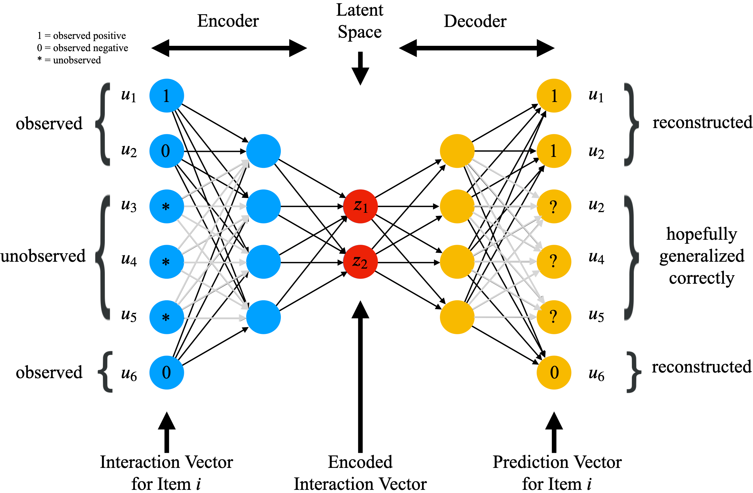
One important advantage of these autoencoder approaches, assuming that they are trained on user-interaction vectors, is that they can achieve strong generalization (as explained the work of [40]), since they may do predictions for a user or item interaction vector that was not observed at training time, whereas all the approaches that we have seen so far always relied on having a pre-trained embedding vector for each user and item.

Similarly as with matrix factorization, the major challenge in these autoencoder approaches is that for typical recommender system datasets the input vectors are extremely sparse, inhibiting to get informative gradients [41]. One of the first papers applying autoencoders to collaborative filtering was the one by Sedhain et al., proposing the architecture Autorec[42]. Autorec computes the reconstruction of an input $\vx\in\R^d$, that can be either a user- or an item-interaction vector, via a shallow autoencoder

$$h(\vx;\vtheta) = f(\MW g(\MV\vx +\vmu)+\vb),$$

where $f$ and $g$ are element-wise activation functions. The objective trained to optimize Autorec’s parameters $\vtheta$ is

where $\norm{\argdot}_{\cO}$ means that gradient-updates are only computed to parameters that are connected to the observed entries of the interaction vector $\vx$. So, actually there exist two versions of Autorec: $U$-Autorec and $I$-Autorec. They differ by the training examples that they consider: $U$-Autorec uses user-interaction vectors $\cS_U=\set{\vx_u}_{u\in\U}$ and $I$-Autorec uses item-interaction vectors $\cS_I=\set{\vx_i}_{i\in I}$. The training/validation/test-split was done by doing a random 80%/10%/10%-split of the interactions. In the case of $I$-Autorec, the prediction of the relevance of item $i$ for a a user $u$ is done through

$$\hat{x}_{ui}=(h(\vx_i))_u.$$

The architecture and gradient-updates with $I$-Autorec are illustrated in the following picture.

In their experiments, Sedhain et al. noticed that $I$-Autorec performed better than $U$-Autorec and argued that this had to do with the fact that, in their considered datasets, the item-interaction vectors were denser than the user-interaction vectors, leading to more reliable predictions. While they do not state this explicitly, one may also believe that using the denser item-interaction vectors also leaded to more and better gradients, since more inputs are non-zero. In Sedhain et al.’s experiments Autorec outperformed classical matrix factorization methods, motivating the use of autoencoders. Preliminary experiments also revealed that deeper autoencoders perform better.

The paper from Strub & Mary [41] then was one of the first autoencoder approaches for collaborative filtering to explicitly state the sparsity problem and to concretely tackle it with an approach. Strub & Mary also trained a loss similar to the masked squared reconstruction loss as Sedhain et al., with two important differences:

• They did not just consider the reconstruction error, but the prediction error for a held-out item, therefore changing the reconstruction target by the additional target item entry.

• They applied masking noise to the input interaction vectors to have the autoencoder learn to reconstruct interactions.

In their experiments, Strub & Mary also showed that autoencoders can outperform state-of-the-art recommender baselines.

Inspired by $I$-Autorec [42] and the approach of Strub & Mary [41], Kuchaiev & Ginsburg [43] from NVIDIA came along with further improvements and another solution to tackle the sparsity problem. Kuchaiev & Ginsburg used a technique called dense re-feeding to deal with the the natural sparsity of the interaction vectors. With dense re-feeding the output $h(\vx)$, that is considered to be denser since it is a probability-distribution, is re-fed to the autoencoder as an input, and is just re-considered as a new training example with the same original target. Their argument for using $h(\vx)$ again as an input is that $h(\vx)$ should represent a fixed-point of the autoencoder: $h(h(\vx))=h(\vx)$. Kuchaiev & Ginsburg mention that the dense re-feeding could be repeated several times, but they only applied it once. A further improvement that Kuchaiev & Ginsburg did, is to use a time-based training/validation/test-split, motivated by the fact that the recommender system should predict future ratings from past ones, rather than randomly missing ratings (as opposed to the splits used in [42, 41]). In their experiments, Kuchaiev & Ginsburg observed that deeper autoencoders with SELU activation functions and a high dropout-rate (e.g., 0.8), where dropout is only used on the latent representation, trained together with dense re-feeding performed the best. An important remark here is that one should not apply dropout on the initial layer, as happening with the masking noise of Strub & Mary, if one does not want the recommender system to learn to predict any random missing rating (e.g., correlations between items), but rather a future rating.

Recently, Liang et al. from Netflix [40] came along and extended variational autencoders (VAEs) to collaborative filtering. Their generative model uses a multinomial likelihood, with the motivation that is better-suited for modeling implicit feedback data, since it is a closer proxy to the ranking loss compared to the more popular likelihood functions such as the multivariate Gaussian (induced by squared loss) and logistic loss.

The entire VAE architecture is then given by the encoder $g_{\phi}$ and decoder $f_{\theta}$ as

The VAE is trained by annealing the evidence lower bound (ELBO)

where $\beta$ is chosen to be $\beta<1$, relaxing the prior constraint that

$$\frac{1}{\card{U}}\sum_{u\in U} \cDist{q_{\phi}}{\vz_u}{\vx_u} \approx p(\vz)=\cN(\vz;\vo,\MI)$$

and sacrificing the ability to good ancestral sampling. Anyways, Kuchaiev & Ginsburg argue that ancestral sampling is not needed in collaborative filtering. Therefore, the prediction is simply performed by using the mean $\mu_{\phi}(\vx_u)$ in the forward propagation, without any sampling of $\epsilon$, giving

$$\hat{\vx}_u=f_{\theta}(\vmu_{\phi}(\vx_u)).$$

In their experiments Liang et al. showed that the Multinomial likelihood yields slightly better results than the Gaussian and the logistic likelihood. Further, they showed that their architecture outperforms several state-of-the-art baselines.

Let us conclude the presentation of autoencoders for collaborative filtering with two properties that all autoencoder approaches have in common: One advantage of all autoencoder approaches is that they do not need any negative sampling. One major disadvantage of all the autoencoder approaches is that, inherently, depending on whether they are item-based or user-based, they either predict the relevance of all $\card{I}$ items for a user, or the relevance to all $\card{U}$ users of an item. This means that the input/output dimensions of the autoencoders are always at least $\min(\card{U},\card{I})$. Thus, they do not scale to datasets with a massive amount of users and items. Also, their latent representations are hard to interpret and it’s not clear how to perform efficient nearest-neighbour searches as one could do with LSH.

Summary of Presented Collaborative Filtering Approaches

Let’s recap on a high-level what the various recommender system approaches do in order to generalize to recommendations on unseen interactions:

• Item Popularity: recommends items based on their popularity. The hope is that the prediction through the popularity of items generalizes to the relevances of unseen user-item pairs.

• Matrix Factorization: learns embeddings that are fed through a bi-linear interaction function, the dot product, to predict the rankings. The hope is that the dot-product of embedding vectors of unseen user-item pairs generalizes to the true relevances.

• Metric Learning Approaches: learn user and item embeddings in a metric spaces such that the distance is correlated with the relevance between users and items. Using a distance metric allows to exploit the phenomenon of similarity propagation. The hope is that the distances between the learned embeddings generalize to the true distances between unseen user-item pairs.
  • Collaborative Metric Learning: uses Euclidean metric space
  • Hyperbolic Recommender Systems: use hyperbolic metric spaces

• Neural Collaborative Filtering: learns embeddings and the parameters of a non-linear interaction function, that is a joint model of a shallow generalized matrix factorization and a pyramidal MLP, to predict the rankings. The hope is that the predictions of rankings through this non-linear interaction function with the learned embeddings generalize well for unseen user-item pairs.

• Autoencoder Approaches: can be seen as non-linear matrix factorization. They learn a non-linear mapping from user (or item) interaction vectors to a latent representation, or distribution, from which other relevant items will be predicted through a non-linear decoding function that gives the relevances of, or a relevance-distribution over, the items (or users for an item). The hope is that the encoding and decoding of (unseen) interaction vectors gives the right relevance predictions for the yet unobserved entries.

References

1. “How retailers can keep up with consumers.” https://www.mckinsey.com/industries/retail/our-insights/how-retailers-can-keep-up-with-consumers.
2. “Understanding Spotify: Making Music Through Innovation.” https://www.goodwatercap.com/thesis/understanding-spotify, 2018.
3. J. Bennett, S. Lanning, and others, “The netflix prize,” in Proceedings of KDD cup and workshop, 2007, vol. 2007, p. 35.
4. C. A. Gomez-Uribe and N. Hunt, “The netflix recommender system: Algorithms, business value, and innovation,” ACM Transactions on Management Information Systems (TMIS), vol. 6, no. 4, p. 13, 2016.
5. Y. Koren, R. Bell, and C. Volinsky, “Matrix factorization techniques for recommender systems,” Computer, no. 8, pp. 30–37, 2009.
6. Y. Koren, “The bellkor solution to the netflix grand prize,” Netflix prize documentation, vol. 81, no. 2009, pp. 1–10, 2009.
7. “Netflix Recommendations: Beyond the 5 stars (Part 1).” https://medium.com/netflix-techblog/netflix-recommendations-beyond-the-5-stars-part-1-55838468f429, 2012.
8. Y. Hu, Y. Koren, and C. Volinsky, “Collaborative filtering for implicit feedback datasets,” in 2008 Eighth IEEE International Conference on Data Mining, 2008, pp. 263–272.
9. C.-K. Hsieh, L. Yang, Y. Cui, T.-Y. Lin, S. Belongie, and D. Estrin, “Collaborative metric learning,” in Proceedings of the 26th international conference on world wide web, 2017, pp. 193–201.
10. G. Adomavicius and A. Tuzhilin, “Context-aware recommender systems,” in Recommender systems handbook, Springer, 2011, pp. 217–253.
11. D. W. Oard, J. Kim, and others, “Implicit feedback for recommender systems,” in Proceedings of the AAAI workshop on recommender systems, 1998, vol. 83.
12. J. Davidson et al., “The YouTube video recommendation system,” in Proceedings of the fourth ACM conference on Recommender systems, 2010, pp. 293–296.
13. H.-T. Cheng et al., “Wide & deep learning for recommender systems,” in Proceedings of the 1st workshop on deep learning for recommender systems, 2016, pp. 7–10.
14. J. L. Bentley, “K-d trees for semidynamic point sets,” in Proceedings of the sixth annual symposium on Computational geometry, 1990, pp. 187–197.
15. A. Shrivastava and P. Li, “Asymmetric LSH (ALSH) for sublinear time maximum inner product search (MIPS),” in Advances in Neural Information Processing Systems, 2014, pp. 2321–2329.
16. A. Gionis, P. Indyk, R. Motwani, and others, “Similarity search in high dimensions via hashing,” in Vldb, 1999, vol. 99, no. 6, pp. 518–529.
17. S. Har-Peled, P. Indyk, and R. Motwani, “Approximate nearest neighbor: Towards removing the curse of dimensionality,” Theory of computing, vol. 8, no. 1, pp. 321–350, 2012.
18. M. Bawa, T. Condie, and P. Ganesan, “LSH forest: self-tuning indexes for similarity search,” in Proceedings of the 14th international conference on World Wide Web, 2005, pp. 651–660.
19. B. Sarwar, G. Karypis, J. Konstan, and J. Riedl, “Application of dimensionality reduction in recommender system-a case study,” Minnesota Univ Minneapolis Dept of Computer Science, 2000.
20. Y. Koren, “Factorization meets the neighborhood: a multifaceted collaborative filtering model,” in Proceedings of the 14th ACM SIGKDD international conference on Knowledge discovery and data mining, 2008, pp. 426–434.
21. R. Pan et al., “One-class collaborative filtering,” in 2008 Eighth IEEE International Conference on Data Mining, 2008, pp. 502–511.
22. X. He, H. Zhang, M.-Y. Kan, and T.-S. Chua, “Fast matrix factorization for online recommendation with implicit feedback,” in Proceedings of the 39th International ACM SIGIR conference on Research and Development in Information Retrieval, 2016, pp. 549–558.
23. A. Mnih and R. R. Salakhutdinov, “Probabilistic matrix factorization,” in Advances in neural information processing systems, 2008, pp. 1257–1264.
24. Y. Zhou, D. Wilkinson, R. Schreiber, and R. Pan, “Large-scale parallel collaborative filtering for the netflix prize,” in International conference on algorithmic applications in management, 2008, pp. 337–348.
25. Y. Koren, “Collaborative filtering with temporal dynamics,” in Proceedings of the 15th ACM SIGKDD international conference on Knowledge discovery and data mining, 2009, pp. 447–456.
26. L. Xiong, X. Chen, T.-K. Huang, J. Schneider, and J. G. Carbonell, “Temporal collaborative filtering with bayesian probabilistic tensor factorization,” in Proceedings of the 2010 SIAM international conference on data mining, 2010, pp. 211–222.
27. X. Luo, M. Zhou, Y. Xia, and Q. Zhu, “An efficient non-negative matrix-factorization-based approach to collaborative filtering for recommender systems,” IEEE Transactions on Industrial Informatics, vol. 10, no. 2, pp. 1273–1284, 2014.
28. Q. Gu, J. Zhou, and C. Ding, “Collaborative filtering: Weighted nonnegative matrix factorization incorporating user and item graphs,” in Proceedings of the 2010 SIAM international conference on data mining, 2010, pp. 199–210.
29. J. Mairal, F. Bach, J. Ponce, and G. Sapiro, “Online learning for matrix factorization and sparse coding,” Journal of Machine Learning Research, vol. 11, no. Jan, pp. 19–60, 2010.
30. H. Dadkhahi and S. Negahban, “Alternating Linear Bandits for Online Matrix-Factorization Recommendation,” arXiv preprint arXiv:1810.09401, 2018.
31. H. Wang, Q. Wu, and H. Wang, “Factorization bandits for interactive recommendation,” in Thirty-First AAAI Conference on Artificial Intelligence, 2017.
32. S. Rendle, C. Freudenthaler, Z. Gantner, and L. Schmidt-Thieme, “BPR: Bayesian personalized ranking from implicit feedback,” in Proceedings of the twenty-fifth conference on uncertainty in artificial intelligence, 2009, pp. 452–461.
33. X. He, L. Liao, H. Zhang, L. Nie, X. Hu, and T.-S. Chua, “Neural collaborative filtering,” in Proceedings of the 26th international conference on world wide web, 2017, pp. 173–182.
34. M. Cogswell, F. Ahmed, R. Girshick, L. Zitnick, and D. Batra, “Reducing overfitting in deep networks by decorrelating representations,” arXiv preprint arXiv:1511.06068, 2015.
35. T. D. Q. Vinh, Y. Tay, S. Zhang, G. Cong, and X.-L. Li, “Hyperbolic recommender systems,” arXiv preprint arXiv:1809.01703, 2018.
36. B. P. Chamberlain, S. R. Hardwick, D. R. Wardrope, F. Dzogang, F. Daolio, and S. Vargas, “Scalable Hyperbolic Recommender Systems,” arXiv preprint arXiv:1902.08648, 2019.
37. T. Schmeier, J. Chisari, S. Garrett, and B. Vintch, “Music recommendations in hyperbolic space: an application of empirical bayes and hierarchical poincaré embeddings,” in Proceedings of the 13th ACM Conference on Recommender Systems, 2019, pp. 437–441.
38. K. Liu and P. Natarajan, “WMRB: Learning to Rank in a Scalable Batch Training Approach,” arXiv preprint arXiv:1711.04015, 2017.
39. M. Nickel and D. Kiela, “Poincaré embeddings for learning hierarchical representations,” in Advances in neural information processing systems, 2017, pp. 6338–6347.
40. D. Liang, R. G. Krishnan, M. D. Hoffman, and T. Jebara, “Variational autoencoders for collaborative filtering,” in Proceedings of the 2018 World Wide Web Conference, 2018, pp. 689–698.
41. F. Strub and J. Mary, “Collaborative filtering with stacked denoising autoencoders and sparse inputs,” 2015.
42. S. Sedhain, A. K. Menon, S. Sanner, and L. Xie, “Autorec: Autoencoders meet collaborative filtering,” in Proceedings of the 24th International Conference on World Wide Web, 2015, pp. 111–112.
43. O. Kuchaiev and B. Ginsburg, “Training deep autoencoders for collaborative filtering,” arXiv preprint arXiv:1708.01715, 2017.